EXPLORING SCALE EFFECT USING GEOGRAPHICALLY WEIGHTED
REGRESSION ON MASS DATASET OF URBAN ROBBERY
Ö. Yavuz a,
*, V. Tecim b
a Department of Geographical Information Systems, The Graduate School of Natural and Applied Sciences, Dokuz Eylul University 35160 Buca Izmir, Turkey - [email protected]
b Department of Econometrics, Faculty of Economics and Administrative Sciences, Dokuz Eylul University, 35160 Buca Izmir, Turkey - [email protected]
KEY WORDS: GIS, Urban, Spatial, Information, Analysis, Exploration
ABSTRACT:
Urban geographers have been studying to explain factors influencing crime on cases limited by their study areas. Researchers have a common opinion that explanatory variables modelling crime on those cases might be irrelevant for another one. None of the researchers tested significance of these variables with changing scales of the study area. Because their data did not allow them to study with different scales. This research examines the scale effect with various data from a wide range of data sources. Geographically Weighted Regression (GWR) method is used to explain that effect, after organizing data by Geographical Information System (GIS) technologies. Explanatory variables deduced for district scale are different from those for grid scale. Hence, the explanatory variables may change not only for different geographical areas but also for different scales of the same area.
* Corresponding author.
1. INTRODUCTION
An increasing number of big cities cause social, cultural and economic interactions between inhabitants. People may interact with each other in negative way and crime is one of them. Various crime types like robbery, assault, etc. rise with the increase of population and interactions (Ackerman, 1998; General Police Department of Anti-Smuggling and Organized Crime, 2012). Much research focuses on explaining the quantitative increase of crime by using data in order to provide more secure cities. Mass dataset from a wide range of data sources calls for managing various data formats. Hence, mass data can help explain crime by identifying crime patterns. Because “place” plays a vital role in understanding crime (Chainey & Ratcliffe, 2005), earlier studies focused on visual presentation of crime to look for patterns in the crime data, namely crime mapping. Crime events are not distributed randomly in space (Brantingham & Brantingham, 1997; Alpdemir & Çabuk, 2005), various factors can influence crime occurrences. Therefore just a crime mapping cannot be enough to provide crime prevention, identification and mapping of the factors is essential as well. Hence, urban geographers studied the ecology of crime that is, the relationship between crime, the built environment, land use etc. (Olligschlaeger, 1997).
According to socioeconomic findings of many ecology studies since 1960s, crimes are highly correlated with poverty (Gorr & Olligschlaeger, 1994; Olligschlaeger, 1997; Cahill & Mulligan, 2003; Ceccato et al., 2002; Gruenewald et al., 2006), unemployment (Schmid, 1960; Ackerman, 1998; Ceccato et al., 2002; Gruenewald et al., 2006), lower income (Schmid, 1960; Ackerman, 1998), education levels (Schmid, 1960; Ackerman, 1998; Cahill & Mulligan, 2003; Cozens, 2002; Gruenewald et al., 2006), being a renter (Ackerman, 1998), population density (Ackerman, 1998; Cahill & Mulligan, 2003; Ceccato et al., 2002; Cozens, 2002; Malczewski & Poetz, 2005), migration (Ackerman, 1998; Ceccato et al., 2002), minority (Ackerman,
1998; Gruenewald et al., 2006), marital status (Ackerman, 1998), number of children (Ackerman, 1998; Olligschlaeger, 1997; Gruenewald et al., 2006), youth (Olligschlaeger, 1997; Gruenewald et al., 2006), family structure (Cahill & Mulligan, 2003; Ceccato et al., 2002; Malczewski & Poetz, 2005), ethnicity (Ergün & Yirmibeşoğlu, 2005; Gruenewald et al., 2006) and commercial land uses (Olligschlaeger, 1997; Cozens, 2002; Ergün & Yirmibeşoğlu, 2005).
These socioeconomic variables change slowly over time and cannot explain short-term variations in crime rates. However daily and hourly fluctuations in crime are far more variable than year to year shifts (Cohn, 1990). In this manner spatiotemporal variables are investigated that might also lead to an increasing number of crime. The studies, conducted in 1980s, found significant linear relationships between ambient temperature and crime (Anderson & Anderson, 1984; Cohn, 1990; Field, 1992; Salleh et al., 2012). According to Cohn (1990) patterns in the crime rate are also linked to temporal and ecological factors like surface temperature, sunlight, rain and wind because these factors induce stress and discomfort among inhabitants which are related to crime occurances (Salleh et al., 2012).
Not only weather but also physical environment has certain magnitude towards the level of human behaviour (Cohn, 1990; Field, 1992). Some geographical findings reveal that crimes are considerably correlated with distance from city center (Ceccato et al., 2002; Ergün & Yirmibeşoğlu, 2005), accessibility (Ceccato et al., 2002; Ergün & Yirmibeşoğlu, 2005), design of a housing (Newman, 1972; Ceccato et al., 2002; Cozens, 2002), number of public transportation (Murray et al., 2001; Ayhan, 2007), building environments (Newman, 1972; Ayhan, 2007).
the factors influencing crime patterns. Geographical Information System (GIS) technologies enable to store, manage and visualize both spatial and non-spatial data (Longley et al., 2001; Tecim, 2008) to extract information from mass data (Thurston, 2002). GIS has capability to associate many forms of information derived from various data sources with specific locations (Taylor & Blewitt, 2006) and provide continuous interaction with data to users. Therefore, GIS technologies have been used in ecology of crime studies.
Above cited studies aim to understand crime occurrences by using spatial analysis techniques such as weighted spatial adaptive filtering (Gorr & Olligschlaeger, 1994), chaotic cellular forecasting (Olligschlaeger, 1997), Getis-Ord statistics (Murray et al., 2001; Ceccato et al., 2002; Gruenewald et al., 2006), Geographically Weighted Regression (GWR) (Malczewski & Poetz, 2005) or non-spatial analysis techniques such as linear regression (Ackerman, 1998; Ayhan, 2007) and correlation analysis (Ergün & Yirmibeşoğlu, 2005; Salleh et al., 2012). Some of them focused on street level crime explanation like Gorr & Olligschlaeger (1994) and Ayhan (2007), whereas some of them studied on city or district level like Schmid (1960) and Ackerman (1998).
Researchers used data to explain crime on cases limited by their study areas, so inferences are only limited to those areas. This limitation about explaining the crime events of spatial study area is an important consequence of the Modifiable Areal Unit Problem (MAUP). The use of different areal units may have influence on the results of ecology of crime studies (Openshaw, 1984). Although studies explain crime by several variables, these explanatory variables are not identical for each case and they are variable from country to country or even from region to region in a country. In addition, to our knowledge no study attempts to make inferences on same study area by changing the scale and thus changing the significance of explanatory variables.
In this research, we investigate whether the same set of variables explain the robbery events for two different scales. Socioeconomic, spatiotemporal and geographical explanatory variables are identified at district and grid scales of the study area by using Geographically Weighted Regression (GWR). GWR allows different relationships to exist at different points in space by calibrating a multiple regression model and investigate local trends in nonstationarity in regression models (Brunsdon et al., 1996). Hence, this research performed on Izmir that is world’s one of the urban agglomerations (UN, 2011), to determine if the explanatory variables changes with changing scale of the study area by using socioeconomic, spatiotemporal and geographical variables.
2. METHODOLOGY
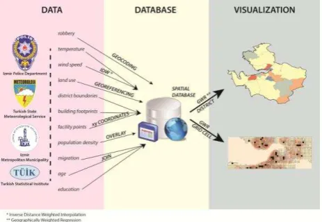
Various types of data in the urban area of Izmir are obtained from different data sources covering the full month of August 2010. Auguts is the mostly reported season of robberies, which also applies for our case in this study (Salleh et al., 2012). The methodology comprises organization of acquired data and design of organized data to make it appropriate for using both district and grid scale of the study area. GIS technologies are used to organize, store and visualize data with the help of integrating information from a variety of sources into one user interface (Olligschlaeger, 1997). All existing data were transformed to a spatial database in order to carry out spatial
query and analysis. The arrows in Figure 1 are labelled with the methods used.
Figure 1. Organization, storage and visualization of data with using adopted methods
Data containing 1344 robbery events used in this research were obtained from Izmir Police Department in a spreadsheet format. The data consist of date, time, crime types and geographical locations of the events. The robbery events were already geocoded by the Police Department from address information of the events.
Independent variables such as socioeconomic, spatiotemporal and/or geographical are essential to explain robbery. Meteorological data were chosen for the spatiotemporal variable according to the background of this research. Totally 6 meteorology stations are located across the study area. Station data with approximately 1464 records in spreadsheet format is obtained from Turkish State Meteorological Service including station names, date, time, temperature, wind speed and address information. The dataset was only restricted to temperature and wind speed since no rain event was observed during the study period. The stations were not equipped with sensors measuring other meteorological observables.
Meteorology stations consist of discrete locations in the study area. As Brunsdon et al. (2001) mentioned although there was a point data over sparse networks, it is useful to interpolate these records as a continuous surface. By Inverse Distance Weighted Interpolation (IDW), we created continuous surface maps for temperature and wind speed using observations at meteorological stations according to Equation 1.
Zj = the temperature/wind speed at sampled location j dij = the distance from i to j
k = the inverse distance weighting power (k=2)
Meteorology stations collect temperature and wind speed values in every one hour period. However, meteorological data have
critical changes that occur at 07:00 (morning), 14:00 (noon) and 21:00 (night) (Turkish State Meteorological Service, 2012). So that IDW method is applied to temperature and wind speed values of every day between 1st and 31st of August 2010 at morning, evening and night respectively (see Appendix 1). Result of this method produces raster based map. Each pixel of raster map contains point data of robbery to assign values to each robbery events.
As a geographical variable of the study, point data of facilities are provided by Izmir Metropolitan Municipality. Data include gas stations, public transportation locations (bus stations, terminal, gang board, etc.), self-help centers, banking, police stations, military and recreation sites besides religious, educational, industrial, commercial, social, cultural, historical and tourist facilities and government agencies. These intense data consist of 4632 individual facility points.
Figure 2. Overlay of robbery events with trade (banking and commercial facility locations), education and public
transportation stations
We selected those facilities covering almost all crime locations by setting the buffer distance of 150 meters. This distance value is selected empirically by increasing the distance at 50 metres intervals. The facilities not fulfilling the above buffer criterion are excluded from the analysis. So we obtained that trade (commercial and banking together), education and transportation locations provide best fit for the coverage of the robbery events (see Figure 2). Thus, these facilities with police stations which is the security guard of the city are determined as geographical explanatory variables of the study.
Socioeconomic variables were obtained from census data like district level population, migration, education and age provided by Turkish Statistical Institute. Data extraction is performed by querying the database for primary school graduate of male and 18-35 age male populations. We adopted these queries because robbery events are encountered more frequent among this population group (Turkish Penal Institution, 2008). For grid scale analysis, population data should be calculated for small spatial units. For this purpose, population per building is extracted from vector based building footprints, heights and raster based land use maps of Izmir Metropolitan Municipality.
Land use maps are crucial to identify residential areas in order to calculate individual building populations. Vector maps containing building footprints and heights were overlaid onto land use maps and residential buildings are identified
correspondingly. Other land use types were thus eliminated from the analysis (see Figure 3).
Figure 3. Part of the vector map showing the residential areas and building footprints
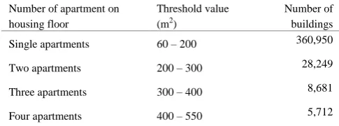
Building footprint size is characteristic for extracting the number of apartments and determining the type of that building also crucial to extract information about the apartment number in a building and usage of a building. For instance, some parcels include residential utility buildings such as garages, sheds and barns (Ural et al., 2011), which are called as “premises”. Because available land use maps show only land use at parcel level, the buildings used as premises inside a parcel cannot be identified. Therefore, area thresholds are applied to classify residential building usages. The area threshold 60 m2 is applied to identify premises. The threshold values for residential buildings are given in Table 1.
Number of apartment on housing floor
Threshold value (m2)
Number of buildings
Single apartments 60 – 200 360,950
Two apartments 200 – 300 28,249
Three apartments 300 – 400 8,681
Four apartments 400 – 550 5,712
Table 1. Threshold values of residential buildings
Height information is necessary to calculate the population per building. The number of households are calculated from mean values of average population per district and building (Ural et al., 2011). The average population density for districts is calculated as 0.26 people/100 m2 and for buildings is 3.49. Mean value of these population densities, which is rounded to two, is taken as constant value of a household number. Population of a building is calculated by multiplying number of households, number of apartments and height of a building. By this methodology the population of the included districts is calculated as 3,364,476 which overlaps with the independently provided district population of 3,479,507 at 96.7 percent level. Therefore, building population is used to calculate population based data in each grid cell.
3. ANALYSIS
Unlike conventional regression, which produces single regression equation to summarize relationships among the explanatory and dependent variables, GWR generates spatial variation in the relationships among variables with producing multiple regression equation (Mennis, 2006). GWR method shows the existence of spatial relationships between different spatial units over space (Brunsdon et al., 1996). To explore scale effect, the spatial relationships between the rate of robbery and four socioeconomic, two spatiotemporal and five geographical variables are included in GWR model. Two different scales, grid and district level, are used for explaining differences and similarities between geographic locations of the robbery events.
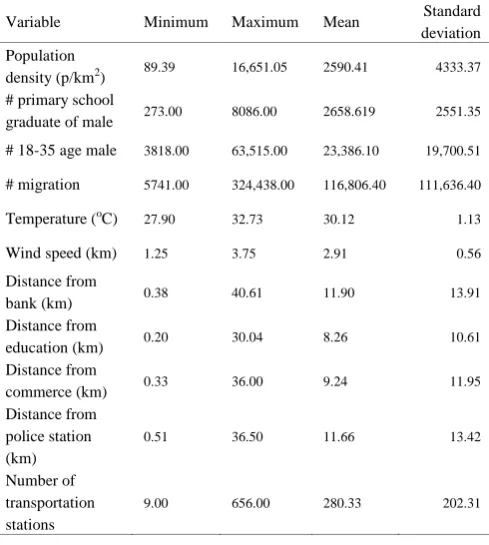
Distances from banking, education, commerce, police station and number of public transportation stations are the geographical variables; temperature and wind speed are the spatiotemporal variables; population density, primary school graduate of male population, 18-35 age male population and migration are the socioeconomic variables of this research. For district scale analysis, descriptive statistics of the variables per district are presented in Table 2.
Variable Minimum Maximum Mean Standard deviation Population
density (p/km2) 89.39 16,651.05 2590.41 4333.37 # primary school
graduate of male 273.00 8086.00 2658.619 2551.35
# 18-35 age male 3818.00 63,515.00 23,386.10 19,700.51
# migration 5741.00 324,438.00 116,806.40 111,636.40
Temperature (oC) 27.90 32.73 30.12 1.13
Table 2. Descriptive statistics for explanatory variables at district scale (n=21)
The population is denser at locations where Izmir bay ends. Some variables such as population density, primary school graduate of male population and number of public transportation stations decrease away from the bay area towards inland. On the other hand the remaining variables increase.
Before constructing GWR model, one of the known linear regression which is Ordinary Least Square (OLS) method is applied to define the significance of explanatory variables in sequential manner. Then, GWR is carried out on robbery data
from 21 district area of Izmir. The separate regression equation for each district is; is the robbery counts in each district
β0 = intercept
Figure 4. Map of GWR at district scale
In Figure 4 deviations from the model in Equation 2 is plotted for each district. Considering the GWR at district scale, distance from education and number of public transportation stations, wind speed and all the socio-economic variables are 95% significantly explain robbery in the study area. At the north and south parts of the study area even 99.5% significant relationship is calculated. At the northwest-southeast direction significance level is partially decreases. On the other hand, some variables like temperature, distances from bank, commerce and police station, has no explanatory significance on robbery at district scale.
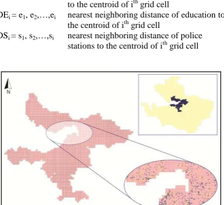
We concentrated our grid scale analysis to the mostly populated area. Determining the explanatory variables of robbery for grid scale, grid cells are used. Grid cell size is defined as 400x400 m and this superimposed on the study area which is shown in Figure 5. This size is not small enough for predicting the future crime with exact location, but it is enough to give an opinion about the risky locations in the study area.
Grid cell midpoint coordinates are used to measure the distance away from the facilities such as DB, DC, DE and DS. NT is the count of the public transportation stations in a grid cell. POP is a total housing population in a grid cell which is computed from land use map per building. SG, AM and M are attained from obtained district level data according to household population in a grid cell. T and W are the averages of assigned robbery meteorology values, respectively.
Grid system is characterized for the grid area as; stations to the centroid of ith grid cell
Figure 5. 400x400m cells for the grid scale area
For grid scale analysis, descriptive statistics of the variables per grid cells are presented in Appendix 2.
Compared to the explanatory variables for district scale, none of the socio-economic variables except population density explains robbery occurrences at grid scale. Contrary to district scale, distances from all facilities are correlated with robbery.
Population density, distances from bank, education, commerce, police station, number of public transportation stations and wind speed are defined as explanatory variables at grid scale (Appendix 3a). These variables explain %35 of the variance in robbery events. By applying spatial autocorrelation (Moran Index) to grid scale, it is obviously seen that robbery counts in grid cell are not distributed randomly over study area (MI=0.32 and Z-score=17.9). "What happens in the local areas surrounding them" are also crucial to identify the relationships existence (Brantingtam & Brantingham, 1997). Kernel density estimation revealed that some robbery events pile up at some locations, which are presented in black colour in Appendix 3b. These locations are the reason of decrease in significance of the explanatory variables.
As Brantingham & Brantingham (1997) mentioned that the occurrence or increase of some crime do not explained with population which is used as dominator. According to our
research robbery events can be explained with dominated population and population related socioeconomic variables at district level. However, at grid scale level dominated geographical variables can explain robbery events. Hence, the research proves that explanatory variables for robbery change with changing scale of the study area.
4. CONCLUSION
An explanatory variable defined for dependent crime value in one of the studies, might be irrelevant for another one. This situation is explained in Fotheringham et al. (2002)’s words as “the measurement of a relationship depends in part on where the measurement is taken”. Actually, obtained data for one set of areal units may not provide the relative significance not only for other study areas but also different scales of the same study area. This research examines if the explanatory variables are changed according to scale effect of the study area. The hypothesis of this research is the dominator of the explanatory variables may change with changing scale of the study area.
To explore the scale effect, district and grid scales of the same study area are used with the help of GWR method. Identifying the differences and similarities of the explanatory variables between two scales, organization of the wide range of data is essential. Most data are obtained in spreadsheet format, and it is crucial to make them spatial. One of the main advantages of an integrated GIS is that all data have one common denominator: the xy coordinates. Thus all data points are related to others via coordinates or the address as well as other characteristics such as the date and time. Then, some adopted methods are applied on data to store them in a spatial database and use for the analysis of this research.
The explanatory variables are defined from three kinds of independent variables which are socioeconomic, spatiotemporal and geographical are performed in GWR model. The results show that population based dominators explain robbery events at district scale. When focused on grid scale, it is seen that these variables are not sufficient to explain robbery events. However, when geographical based dominators are applied in the model, the grid scale results become significant.
5. REFERENCES
Ackerman, V.W., 1998. Socioeconomic correlates of increasing crime rates in smaller communities. Professional Geographer, 50, pp. 372-387.
Alpdemir, A.E. & Çabuk, A., 2005. Eskişehir kenti suç kaynaklarının bilgi sistemleri destekli tespiti ve planlamaya esas teşkil eden verilerle ilişkilendirilmesi. Harita ve Kadastro Mühendisleri Odası, Mühendislik ölçmeleri STB komisyonu, 2. Mühendislik ölçmeleri sempozyumu, İTÜ, 23-25 November 2005. İstanbul.
Anderson, C.A., & Anderson, D.C., 1984. Ambient temperature and violent crime: Tests of the linear and curvilinear hypotheses. Journal of Personality and Social Psychology, 46(1), pp. 91-97.
Ayhan, İ., 2007. Kentte Suç Oranlarının Ekonomik Sosyal ve Mekansal Değişkenlerle Modellenmesi. Thesis of Msc, İzmir: Dokuz Eylül Üniversitesi.
Brantingham, P.L., & Brantingham, P.J., 1997., Mapping crime for analytic purposes: Location quotients, counts, and rates. Crime Mapping and Crime Prevention. New York: Criminal Justice Press, pp. 263-288.
Brunsdon, C., Fotheringham, A.S. & Charlton, M.E., 1996. Geographically weighted regression: A method for exploring spatial nonstationarity. Geographical Analysis, 28(4), pp. 281-298.
Brunsdon, C., McClatchey, J. & Unwin, D.J., 2001. Spatial variations in the average rainfall-altitude relationship in Great Britain: An approach using geographically weighted regression. International Journal of Climatology, 21, pp. 455-466.
Cahill, F.M. & Mulligan, F.G., 2003. The determinants of crime in Tucson, Arizona. Urban Geography, 24, pp. 582-610.
Ceccato, V., Haining, R. & Signoretta, P., 2002. Exploring offence statistics in Stockholm city using spatial analysis tools. Annals of the Association of American Geographers, 92, pp. 29-51.
Chainey, S. & Ratcliffe, J., 2005. GIS and crime mapping. Chichester: Wiley Press.
Cohn, E.G., 1990. Weather and crime. British Journal of Criminology, 30(1), pp. 51-64.
Cozens, P.M., 2002. Sustainable urban development and crime prevention through environmental design for the British city. Towards an Effective Urban Environmentalism for the 21st Century-Cities, 19, pp. 129-137.
Ergün, N. & Yirmibeşoğlu, F., 2005. İstanbul’da 2000-2004 yılları arasında suçun mekansal dağılımı. Planlamada yeni Politika ve Stratejiler Riskler ve fırsatlar: 8 Kasım Dünya Şehircilik Günü 29. Kolokyumu, 7-9 November 2005.İstanbul.
Field, S., 1992. The effect of temperature on crime. British Journal of Criminology, 32(3), pp. 340-351.
Fotheringham, A.S., Brunsdon, C. & Charlton, M., 2002. Geographically Weighted Regression: The Analysis of Spatially Varying Relationships. Chichester: Wiley Press.
General Police Department of Anti-Smuggling and Organized
Crime., 2012.
http://www.kom.gov.tr/Tr/KonuYazdir.asp?CKey=161 (10 Aug. 2012).
Gorr, W.L. & Olligschlaeger, A.M., 1994. Weighted spatial adaptive filtering: Monte Carlo studies and application to illicit drug market modeling. Geographical Analysis, 26, pp. 67-87.
Gruenewald, P.J., Freisthler, B., Remer, L., LaScala, E.A. & Treno, A., 2006. Ecological models of alcohol outlets and violent assaults: Crime potentials and geospatial analysis. Addiction, 101, pp. 666-677.
Longley, P., Goodchild, M., Maguire, D. & Rhind, D., 2001. Geographic Information Systems and Science. Chichester: John Wiley & Sons.
Malczewski, J. & Poetz, A., 2005. Residential burglaries and neighborhood socioeconomic context in London, Ontario:
Global and local regression analysis. The Professional Geographer, 57(4), pp. 516-529.
Mennis, J., 2006. Mapping the results of geographically weighted regression. The Cartographic Journal, 43(2), pp. 171-179.
Murray, T.A., McGuffog, I., Western, S.J. & Mullins, P., 2001. Exploratory spatial data analysis techniques for examining urban crime. British Journal of Criminology, 41, pp. 309-329.
Newman, O., 1972. Defensible Space: Crime Prevention Through Urban Design. New York: Macmillan.
Olligschlaeger, A.M., 1997. Spatial Analysis of Crime Using GIS-Based Data: Weighted Spatial Adaptive Filtering and Chaotic Cellular Forecasting with Applications to Street Level Drug Markets. Thesis of PhD, Pittsburg: Carnegie Mellon University.
Openshaw, S., 1984. The Modifiable Areal Unit P roblem. Norwich: Geo Books.
Salleh, S.A., Mansor, N.S., Yusoff, Z. & Nasir, R.A., 2012. The crime ecology: Ambient temperature vs. spatial setting of crime (burglary). Social and Behavioral Sciences, 42, pp. 212-222.
Schmid, C.F. 1960. Urban crime areas: Part II. American Sociological Review 25, pp. 655-78.
Taylor, G. & Blewitt, G. 2006. Intelligent P ositioning GIS-GPS Unification. Chichester: Wiley Press.
Tecim, V. 2008. Coğrafi Bilgi Sistemleri: Harita Tabanlı Bilgi Yönetimi. Ankara: Renk Form.
Thurston, J., 2002. "GIS and artificial neural networks: Does your GIS think" GIScafe.com(20 May. 2012).
Turkish State Meteorological Service, 2012. Personal interaction (16 Apr. 2012).
Turkish Penal Institution, 2008. "Discharged Convicts Criminal Statistics"
http://tuikapp.tuik.gov.tr/girenhukumluapp/girenhukumlu.zul (12 Jan. 2012).
UN., 2011. "Department of economic and social affairs population division" http://esa.un.org/unpd/wup/CD-ROM/Urban-Agglomerations.htm(20 Nov. 2012).
Ural, S., Hussain, E. & Shan, J., 2011. Building population mapping with aerial imagery and GIS data. International Journal of Applied Earth Observation and Geoinformation, 13, pp. 841-852.
Acknowledgements
We would thank to Izmir Police Department for their help on providing criminal data. And special thanks to Dr. M. Güven KOÇAK for his valuable and constructive suggestions of this research.
Appendix 1. IDW of temperature and wind speed at the urban area in Izmir for the date of 01.08.2010
Appendix 2. Descriptive statistics for independent variables at grid scale (n=1616)
Variable Minimum Maximum Mean Standard deviation
Population density (p/km2) 0 54,417.76 7,550.09 10.28
# primary school graduate of male 0 126.20 17.54 24.69
# 18-35 age male 0 965.96 158.90 211.51
# migration 0 4858.01 760.60 1028.29
Temperature (oC) 23.70 38.20 30.61 1.62
Wind speed (km) 0.60 7.76 3.20 0.77
Distance from bank (km) 0 3805.92 213.79 409.05
Distance from education (km) 0 377.60 15.26 31.50
Distance from commerce (km) 0 1418.95 63.84 160.05
Distance from police station (km) 0 2280.84 199.91 281.57
Number of transportation stations 0 41.00 2.21 2.98
Appendix 3. GWR map of explanatory variables at grid scale
(a) (b)