isprsarchives XXXIX B3 1 2012

EVALUATION OF PENALTY FUNCTIONS FOR SEMI-GLOBAL MATCHING

COST AGGREGATION

Christian Banz, Peter Pirsch, and Holger Blume

Institute of Microelectronic Systems Leibniz Universität Hannover, Hannover, Germany

④❜❛♥③✱♣✐rs❝❤✱❜❧✉♠❡⑥❅✐♠s✳✉♥✐✲❤❛♥♥♦✈❡r✳❞❡

KEY WORDS:Stereoscopic, Quality, Matching, Vision, Reconstruction, Camera, Disparity Estimation, Semi-Global Matching

ABSTRACT:

The stereo matching method semi-global matching (SGM) relies on consistency constraints during the cost aggregation which are enforced by so-called penalty terms. This paper proposes new and evaluates four penalty functions for SGM. Due to mutual depen-dencies, two types of matching cost calculation, census and rank transform, are considered. Performance is measured using original and degenerated images exhibiting radiometric changes and noise from the Middlebury benchmark. The two best performing penalty functions are inversely proportional and negatively linear to the intensity gradient and perform equally with 6.05 % and 5.91 % average error, respectively. The experiments also show that adaptive penalty terms are mandatory when dealing with difficult imaging condi-tions. Consequently, for highest algorithmic performance in real-world systems, selection of a suitable penalty function and thorough parametrization with respect to the expected image quality is essential.

1 INTRODUCTION

Calculating depth information by stereo matching (disparity esti-mation) is a common image processing task in many remote sens-ing applications. Typical applications of range cameras based on stereo imaging include advanced driver assistance systems, robotics, and keyhole surgery assistance systems. Crucial aspects for real-world suitability is accuracy and density of the depth map, which are especially difficult to achieve at in untextured areas. These requirements are further impacted by noise and dif-ficult lighting conditions. Naturally, all of these effects occur in real-world scenarios.

The semi-global matching algorithm (SGM) (Hirschmüller, 2008) is among the top-performing algorithms in the ongoing Middle-bury benchmark (Scharstein and Szeliski, 2012). The benchmark originated from the studies in (Scharstein and Szeliski, 2002) comparing state-of-the-art stereo methods using a controlled set of test images with complex scene structure and varying texture. It has also been shown that SGM is able to effectively deal with the aforementioned issues (Hirschmüller and Scharstein, 2009). Several combinations of matching cost functions and stereo meth-ods were evaluated using original and degraded test images (e. g. noise, exposure differences).

Furthermore, it has recently been shown that SGM can be im-plemented in real-time on a variety of platforms. For example, an FPGA implementation (Banz et al., 2011b) and a GPU

imple-mentation (Banz et al., 2011a) both reach over60fps for VGA

images with 128 pixel disparity range. The high algorithmic per-formance and real-time capability make SGM very attractive for a wide range of applications including low power embedded vision systems and desktop system with off-the-shelf hardware.

Of major relevance to the performance are the smoothness con-straints that are imposed by SGM during the cost aggregation step. These constraints are adapted to the image content by means of so-called penalty functions which penalize abrupt changes in the depth information when, according to image content, a change of objects is unlikely. Therefore, the choice of penalty functions has a significant influence on the algorithmic performance and

robustness. Despite the many surveys on SGM, the influence of the penalty functions has not yet been investigated.

In this paper, new penalty functions for the cost aggregation step of SGM are proposed and evaluated. Due to the mutual depen-dency of matching cost function and penalty function, two match-ing cost functions for initial correspondence hypothesis are con-sidered. These are based on the rank transform and the census transform (Zabih and Woodfill, 1994), both of which are often used in systems for disparity estimation due to their good perfor-mance and efficient implementation possibilities. Each penalty function is parametrized for both matching cost functions us-ing the established data sets with ground truth disparities from (Scharstein and Szeliski, 2002) with and without additional con-trolled radiometric changes of intensity similar to (Hirschmüller and Scharstein, 2009) as well as noise. Evaluation is performed in terms of, firstly, accuracy and density of the disparity map and, secondly, the insensitivity to the degraded input images.

Section 2 reviews algorithmic background on semi-global match-ing and disparity estimation. Section 3 details the methodology, experiments and results for the different test sets. Conclusions are drawn in Section 4.

2 STEREO MATCHING

It is important to distinguish between the initial a similarity mea-sure (matching costs) between two pixels in the base and match image (or left and right image, respectively) and the aggregation method that uses these costs. In this work, rank transform and census transform (Zabih and Woodfill, 1994) are considered as matching costs functions and semi-global matching (Hirschmüller, 2008) is used for cost aggregation. Final disparity selection is performed by a winner-take-all (WTA) approach.

2.1 Rank Transform

Matching costsC(p, d)based on the rank transform (RT) of the

base and match imageRbandRmare calculated as

y

Figure 1: Investigated path orientations for eight and four paths.

wherep = [px, py]Tis the pixel location in the left image and

Ris the area-based non-parametric rank-transform. It is defined

as the number of pixelsp′in a squareM ×M (here: M= 9)

neighborhoodA(p)of the center pixelpwith a luminous

inten-sityIless thanI(p)

neighborhoodA(p)of the center pixelpto a bit string where

pix-els with an intensityIless thanI(p)are1, else0. Thus,

R(p) = ⊗

p′∈A(p)

ξ I(p′), I(p) (3)

with⊗the concatenation andξ(a, b) = 1 ∀ a < b, 0 else.

The matching cost between two pixels is the Hamming distance of the corresponding census transformed pixels, i. e.

C(p, d) =

whereiindexes the bit position. The census transform is also

non-parametric and area based.

Both methods are able to deal with radiometric differences since they depend on the ordering of the pixel’s intensities rather than the absolute values. In contrast to the rank transform, spatial in-formation is retained by the census transform.

2.3 Semi-Global Matching

In many cases, pixel-wise calculated matching costs (i.e. locally calculated) yield non-unique or wrong correspondences due to low texture and ambiguity. Therefore, semi-global matching in-troduces global consistency constraints by aggregating matching costs along several independent, one-dimensional paths across the image. Thereby, SGM aims to approximate a global energy minimization problem which is NP-hard. The paths are

formu-lated recursively by the definition of the path costsLr(p, d)along

a pathr.

The first term describes the initial matching costs. The second

term adds the minimal path costs of the previous pixelp−r

including a penaltyP1 for disparity changes andP2for

dispar-ity discontinuities, respectively. Discrimination of small changes

|∆d|= 1pixel (px)and discontinuities|∆d|>1px allows for

slanted and curved surfaces on the one hand and preserves dis-parity discontinuities on the other hand. The last term prevents constantly increasing path costs. For a detailed discussion refer to

(Hirschmüller, 2008).P1is an empirically determined constant.

0 10 20 30 40 50 60 70

Figure 2: Matching costs, aggregated path costs, and sum costs

for the pixelp= [183; 278]of the Teddy image calculated with

census transform and SGM.

P2can also a empirically determined constant or can be adapted

to the image content. The selection of these penalty functions is focus of this contribution and will be discussed in 3 in detail.

Quasi-global optimization across the entire image is achieved by calculating path costs from multiple directions to a pixel, as shown

in Fig. 1. The aggregated costsSare the sum of the path costs

S(p, d) =

X

r

Lr(p, d). (6)

The disparity mapDb(px, py)from the perspective of the base

camera is calculated by selecting the disparity with the minimal aggregated costs

min

d S(p, d) (7)

for each pixel. For calculatingDm(qx, qy), the minimal

aggre-gated costs along the corresponding epipolar lines are selected:

min

d S(qx+d, qy, d). (8)

The effect of the path costs aggregation and the disparity selec-tion is illustrated in Fig. 2. The initial matching costs (dotted line) exhibit a high level of ambiguity. Seven of the eight aggregated paths costs already show distinct minima. The summed path costs (thick red line) clearly identify the minimum at a disparity level of 32 resolving all ambiguities. However, the cost difference for the positions 32 and 33 is minimal indicating that the correct position is located a sub-pel precision. Half-pel accuracy is obtained by quadratic curve fitting through the neighboring sum costs around the minimum. An evaluation of sub-pel interpolation methods can be found in (Haller and Nedevschi, 2012).

Both, uniqueness check and left/right check are performed to en-sure that only valid disparities with high confidence level are pro-duced. The uniqueness check sets disparities invalid if the

min-imummindS(p, d)is not unique. The left/right-check sets

dis-parities invalid if the disparityDb(p)and its corresponding

dis-parity ofDmdiffer by more than1px. No post-processing steps,

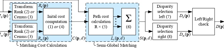
e. g. hole-filling or interpolation, are performed. An overview of the processing steps is given in Fig. 3. From (5) and Fig. 2 the

crucial role of a "‘good"’ selection ofP1 andP2for the overall

performance is obvious. It is suggested in (Hirschmüller, 2008)

to adaptP2(I)to the image content in order to penalize abrupt

disparity changes when, according to image content, a depth dis-continuity is unlikely. Therefore, it is clearly necessary to assess

different functions forP2(I)and their influence on the

Left/Right

Figure 3: Processing steps for disparity estimation using rank transform/census transform and semi-global matching.

3 EVALUATION AND RESULTS

The four evaluated penalty functions are:

(a)empirically determined constant value, i. e.

P2,c=const. (9)

(b)negatively proportional to the absolute luminous intensity

gra-dient of the currently processed pixels along the path, i. e.

P2,l=−α· |I(p)−I(p−r)|+γ (10)

(c)inversely proportional to the absolute luminous intensity

gra-dient of the currently processed pixels along the path. This fol-lows the original proposal from SGM.

P2,i=

α

|I(p)−I(p−r)|+β +γ (11)

(d)negatively proportional to the variance of the luminous

inten-sity in a local window, i. e.

P2,v=−α·Var(A(p)) +γ (12)

In all cases it has to be ensured thatP2≥P1. Therefore, a lower

bound is introducedP2,minto which the values are clipped. An

upper bound is not required because penalty higher thanCmax+

P1 cause that value never to be taken in the outer min-term in

Eq. (5). It follows that (b) does not require a parameterβ for

shift inxdirection. This is implicitly done by adjustingγ. Cases

(b) and (c) are based on the hypothesis that depth changes are often visible as luminance changes. Case (d) is based on the hy-pothesis that matching costs in highly structured areas are highly discriminative and luminance changes not only occur due to ob-ject changes.

3.1 Methodology and Middlebury Images

For the first set of experiments the established Middlebury stereo data set (Cones, Teddy, Venus and Tsukuba) is used (Scharstein and Szeliski, 2002). These were taken under controlled labora-tory conditions. Intensity differences and noise are expected to

be minimal. The disparity ranges are64px for Cones and Teddy,

32 px for Venus, and16 px for Tsukuba. Each penalty function

is parametrized for each image with both matching cost func-tions for 4 and 8 paths. The resulting disparity maps are eval-uated by counting the number of erroneous disparities in non-occluded areas. An erroneous disparity differs by more than a defined threshold from ground truth. Two thresholds are

consid-ered: |∆| >1px and|∆|> 0.5px. Percentages stated in the

following are the number of erroneous pixels of all non-occluded pixels (not the entire image). Ignoring occluded areas, i. e. where disparities cannot be computed, allows to focus on the perfor-mance of the disparity estimation algorithm rather than any post-processing steps. Otherwise, the results would be biased by the

quality of the hole interpolation algorithm. For the same reasons no post-processing steps are applied to the disparity maps.

Questions the first set of experiments is aimed at to answer are: Is there a clear favorite among the penalty functions? How sensi-tive is the performance towards the parametrization of the penalty function? Is the parametrization robust across different images taken with different setups and cameras? These questions are of relevance for real world system since insensitivity towards non-optimal parametrization and camera imposed differences are mandatory.

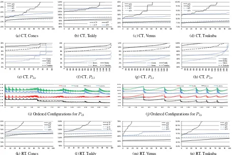
Fig. 4 shows the results computed with census and 8 paths for the four test images as the parametrization of each function is changed. The parameter configurations for each penalty function

are sorted with increasing error and the best100configurations

are shown. The parameters of each function (P1,P2,min,α,β,

andγ) are changed systematically with carefully determined step

sizes big enough to ensure sufficiently different configuration sets on the one hand and small enough not to miss local minima on the other hand.

SettingP2constant performs well if carefully adjusted to the

par-ticular image but quality degrades quickly as these values are

changed. The adaptive functionsP2,l and P2,i perform

signifi-cantly better with up to1percentage points improvement. Both

are comparable in terms of quality and superiority is minimal de-pending on the particular image. The variance based approach performs significantly worse than the other adaptive approaches and sometimes even worse than the fixed approach. This could

be due to the fact thatP2,vdoes not calculate penalties along the

currently processed path but from the local window giving the same penalty value for all path directions. For the census-based

matching costsP2,landP2,iare the best functions.

The second row of Fig. 4 shows the data re-grouped according to penalty function, this time over all configurations analyzed. All functions are insensitive to a certain degree of non-optimal parametrization to the image content. However, it is also clear that good parametrization is essential for obtaining the maximum of correct information.

The third row of Fig. 4 assess if optimal configurations coincide from image to image. The configurations are now ordered ac-cording to the parameter values and same configurations are on the same x-position. Clearly, performance of a particular configu-ration coincides across all images. Further, the best configuconfigu-ration for one image is usually found for the other images when

allow-ing a minimal0.5%percentage point error margin. When going

from 8 paths to 4 paths (data not shown) the same observations and conclusions can be made with just slightly increased error counts. For half-pel error thresholds the are no changes in con-figurations (data not shown).

5.0% Venus Tsukuba

(f) CT,P2,l Venus Tsukuba

(g) CT,P2,i

(i) Ordered Configurations forP2,l

0.0%

(j) Ordered Configurations forP2,i

6.8%

Figure 4: Errors in unoccluded areas for all penalty functions employing census transform examining behavior on the same image (row one), over different images (row two), stability of configurations across images (row three), and employing rank transform (row four).

(a) Left Cones image (b) Ground thruth (c) CT,P2,c (d) CT,P2,l (e) CT,P2,i (f) CT,P2,v

(g) Left Teddy image (h) Ground Truth (i) CT,P2,c (j) CT,P2,l (k) CT,P2,i (l) CT,P2,v

Figure 5: Disparity maps obtained with optimally parametrized penalty functions for Cones (top row) and Teddy (bottom row).

than for the census transform which is due to the missing spatial information of the rank transform. As with the census transform

P2,cperforms acceptably andP2,v poorly for an adaptive

func-tion. However, in opposite to census, P2,l always outperforms

P2,i; in 3 cases quite significantly. All functions are similarly

robust towards parametrization offset as with census (data not shown). Again, good configurations coincide across all images (data not shown).

The error levels obtained with optimally adapted penalty func-tions are summarized in Table 1. For the two test images Cones and Teddy the resulting disparity maps are shown in Fig. 5. Even

visually highly noticeable,P2,vintroduces a significant amount of

errors. UsingP2,ithe small structures in Cones are retained,

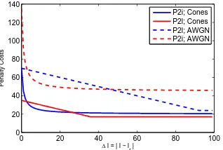
oth-erwise there is no significant difference betweenP2,landP2,i. For

comparison, these two functions are plotted with their optimal configuration in Fig. 6 showing an obvious similarity between

the two functions overx.

3.2 Simulated Degenerated Images

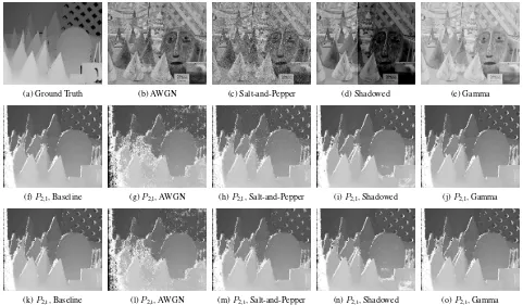
For the second set of experiments the left input image of the Cones data set is artificially degraded whereas the right remains unchanged. Two types of radiometric differences and two types of noise are considered:

• Additive white Gaussian noise (AWGN) with SNR = 12 dB

• Salt-and-Pepper noise with 14 % of the image degenerated

• Linear brightness (gain) change across the half the image

0 20 40 60 80 100 0

20 40 60 80 100 120 140

∆ I = | I − I_r |

Penalty Costs

P2i; Cones P2l; Cones P2l; AWGN P2i; AWGN

Figure 6: Optimal penalty functions (P2,landP2,i) for the Cones

image (solid lines) and in the presence of AWGN (dotted lines).

The degenerated images are shown in Fig. 8 top row. The eval-uation methodology remains as with the first experiments. This experiment is aimed at answering the following questions: Are the penalty functions robust towards a variety of different im-age interferences and which performs best? How robust is the parametrization across these interferences? Is the choice of penalty function and parametrization the same as for the non-degenerated images? The errors curves for the four types of simulated de-generation are shown in Fig. 7. Fixed penalty functions degrade quickly for census and rank, as the constant values are now trained to the type and amount of noise in the image. Adaptive functions are able to cope with the noise and radiometric changes. As with

non-degenerated images,P2,landP2,iperform best and in many

cases similar. For rank,P2,loutperformsP2,iexcept for

salt-and-pepper noise. For census, the two functions perform equally

ex-cept for salt-and-pepper noise where theP2,isignificantly

outper-forms the linear function. The variance based approach is always outperformed by the other adaptive approaches. For qualitative evaluation the resulting disparity maps are shown in Fig. 8.

Comparing configurations across the different types of degener-ation shows that good configurdegener-ations coincide (data not shown). As before, good configurations from one image to the next can often be found within a 0.5 percentage points error margin. How-ever, comparing good configurations to configurations from the non degenerated images shows that now higher dynamic range and higher penalties are chosen. For example, the best

param-eter set from the original Cones image for P2,l is{P1 = 11,

P2,min= 17,γ = 35, α = 0.5}resulting in 5.23 % erroneous

disparities. For the AWGN case it is{P1 = 20, P2,min = 24,

γ= 70,α= 0.5}and for the salt-and-pepper case{P1 = 14, P2,min= 24,γ = 40, α= 0.5}resulting on the original image

in 6.27 % and 5.37 %, respectively. For comparison, the opti-mal penalty functions for the AWGN case have been included in Fig. 6. Consequently, proper selection and parametrization of penalty functions can make disparity estimation robust to high levels of interferences with only minimal performance decrease in ideal cases. However, it also shows that for high-end applica-tions targeting highest quality disparity maps sophisticated image preprocessing is required.

3.3 Real World Images

For real world image data the lack of ground truth makes it ex-tremely difficult to setup automated parametrization. However, optical inspection using real world data from (Ess et al., 2007) was performed with the parametrizations obtained from the non-degenerated and non-degenerated images. Special attention has been paid to planar, little textured areas, edges, and small structures (e. g. lamp posts). Generally, better results were obtained when using the configurations from the degenerated images. This is in accordance with the argumentation from above.

f Cones Teddy Venus Tsukuba

Census Transform

P2,c 5.38 % 10.40 % 2.53 % 8.35 %

P2,l 5.23 % 9.03 % 1.92 % 7.45 %

P2,i 5.43 % 9.30 % 2.06 % 7.55 %

P2,v 5.28 % 10.79 % 2.55 % 8.54 %

Rank Transform

P2,c 7.46 % 12.44 % 4.20 % 9.32 %

P2,l 7.29 % 11.17 % 3.15 % 8.58 %

P2,i 7.37 % 11.76 % 4.13 % 9.06 %

P2,v 7.49 % 12.57 % 4.16 % 9.41 %

Table 1: Errors in non-occluded areas with a threshold of 1 dis-parity obtained with optimally parametrized penalty functions.

f Baseline AWGN Salt Shadow Gamma

Census Transform

P2,c 5.38 % 26.35 % 7.63 % 7.86 % 5.41 %

P2,l 5.23 % 18.91 % 8.27 % 7.27 % 5.27 %

P2,i 5.43 % 18.94 % 7.40 % 7.26 % 5.30 %

P2,v 5.28 % 30.70 % 8.40 % 8.16 % 5.45 %

Rank Transform

P2,c 7.46 % 40.64 % 10.99 % 10.27 % 7.60 %

P2,l 7.29 % 32.61 % 11.74 % 7.27 % 7.41 %

P2,i 7.49 % 40.61 % 11.11 % 9.94 % 7.47 %

P2,v 7.37 % 45.84 % 11.99 % 10.54 % 7.61 %

Table 2: Errors in non-occluded areas with a threshold of 1 dis-parity obtained with optimally parametrized penalty functions on the cones image under various types of degeneration.

4 CONCLUSIONS AND FUTURE WORK

In conclusion, the choice of penalty function and its parametriza-tion has significant influence on the performance of SGM, es-pecially under difficult imaging conditions (e. g. noise, expo-sure differences). While for highly structured images taken

un-der near ideal conditions constant penalty functions (P2,c)

per-form well, they tend to become overfitted to the particular imag-ing conditions and performance is not stable over different

con-ditions. Among the adaptive functions, the linear (P2,l) and

in-versely proportional (P2,i) functions significantly outperform the

variance based approach. They are also robust to interferences in the images making adaptive penalty terms mandatory for ro-bust disparity estimation. Even then, the quality of the dispar-ity map significantly depends on a suitable penalty function for SGM. Using inversely proportional penalty functions, as origi-nally proposed with SGM, does not result in any performance improvement compared to linear dependencies, which is of inter-est for computationally limited implementations. Nevertheless, thorough parametrization according to the employed matching cost function is essential. Since parametrization using difficult images results in more robust parameter sets real world systems should parametrized under these conditions. For all penalty func-tions, employing census transform instead of rank transform ex-hibits better disparity maps with less edge blurring because cen-sus transform retains spatial information. Future work includes testing the penalty functions for other types of matching cost functions, e. g. mutual information.

ACKNOWLEDGEMENTS

15.0%

Figure 7: Errors in unoccluded areas for all penalty functions on degenerated input images employing census and rank transform.

(a) Ground Truth (b) AWGN (c) Salt-and-Pepper (d) Shadowed (e) Gamma

(f)P2,l, Baseline (g)P2,l, AWGN (h)P2,l, Salt-and-Pepper (i)P2,l, Shadowed (j)P2,l, Gamma

(k)P2,i, Baseline (l)P2,i, AWGN (m)P2,i, Salt-and-Pepper (n)P2,i, Shadowed (o)P2,i, Gamma

Figure 8: Degenerated input images (row one) and corresponding disparity maps obtained withP2,l(row two) andP2,i(row three) using

the census transform.

REFERENCES

Banz, C., Blume, H. and Pirsch, P., 2011a. Real-time semi-global matching disparity estimation on the gpu. In: Computer Vision Workshops (ICCV Workshops), 2011 IEEE International Confer-ence on, pp. 514 –521.

Banz, C., Hesselbarth, S., Flatt, H., Blume, H. and Pirsch, P., 2011b. Real-time stereo vision system using semi-global match-ing disparity estimation: Architecture and fpga-implementation. Transactions on High-Performance Embedded Architectures and Compilers, Springer.

Ess, A., Leibe, B. and Van Gool, L., 2007. Depth and appearance for mobile scene analysis. In: IEEE Intl. Conf. Computer Vision, pp. 1 –8.

Haller, I. and Nedevschi, S., 2012. Design of interpolation func-tions for subpixel-accuracy stereo-vision systems. Image Pro-cessing, IEEE Transactions on 21(2), pp. 889 –898.

Hirschmüller, H., 2008. Stereo Processing by Semiglobal Match-ing and Mutual Information. IEEE Trans. Pattern Analysis and Machine Intelligence 30(2), pp. 328–341.

Hirschmüller, H. and Scharstein, D., 2009. Evaluation of

stereo matching costs on images with radiometric differences. IEEE Trans. Pattern Analysis and Machine Intelligence 31(9), pp. 1582–1599.

Scharstein, D. and Szeliski, R., 2002. A taxonomy and evalua-tion of dense two-frame stereo correspondence algorithms. Intl. Journal of Computer Vision 47(1), pp. 7–42.

Scharstein, D. and Szeliski, R., 2012. The Middlebury Stereo Pages. http://vision.middlebury.edu/stereo/.