INFLUENCE OF RIVER BED ELEVATION SURVEY CONFIGURATIONS AND
INTERPOLATION METHODS ON THE ACCURACY OF LIDAR DTM-BASED RIVER
FLOW SIMULATIONS
J. R. Santillan ⃰, J. L. Serviano, M. Makinano-Santillan, J. T. Marqueso
CSU Phil-LiDAR 1 Project, Caraga Center for Geo-informatics, College of Engineering and Information Technology, Caraga State University, Ampayon, Butuan City, Agusan del Norte, Philippines – [email protected],
[email protected], [email protected], [email protected]
KEY WORDS: LiDAR, Digital Terrain Model, River Bed, Survey Configuration, Interpolation, Integration, Flow Simulation
ABSTRACT:
In this paper, we investigated how survey configuration and the type of interpolation method can affect the accuracy of river flow simulations that utilize LIDAR DTM integrated with interpolated river bed as its main source of topographic information. Aside from determining the accuracy of the individually-generated river bed topographies, we also assessed the overall accuracy of the river flow simulations in terms of maximum flood depth and extent. Four survey configurations consisting of river bed elevation data points arranged as cross-section (XS), zig-zag (ZZ), river banks-centerline (RBCL), and river banks-centerline-zig-zag (RBCLZZ), and two interpolation methods (Inverse Distance-Weighted and Ordinary Kriging) were considered. Major results show that the choice of survey configuration, rather than the interpolation method, has significant effect on the accuracy of interpolated river bed surfaces, and subsequently on the accuracy of river flow simulations. The RMSEs of the interpolated surfaces and the model results vary from one configuration to another, and depends on how each configuration evenly collects river bed elevation data points. The large RMSEs for the RBCL configuration and the low RMSEs for the XS configuration confirm that as the data points become evenly spaced and cover more portions of the river, the resulting interpolated surface and the river flow simulation where it was used also become more accurate. The XS configuration with Ordinary Kriging (OK) as interpolation method provided the best river bed interpolation and river flow simulation results. The RBCL configuration, regardless of the interpolation algorithm used, resulted to least accurate river bed surfaces and simulation results. Based on the accuracy analysis, the use of XS configuration to collect river bed data points and applying the OK method to interpolate the river bed topography are the best methods to use to produce satisfactory river flow simulation outputs. The use of other configurations (and a choice between IDW or OK) except RBCL can also be an alternative in cases when the XS configuration is less practical or expensive to implement.
1. INTRODUCTION
The availability of very high spatial resolution topographic datasets from Light Detection and Ranging (LiDAR) technology, particularly Digital Terrain Models (DTMs), has provided flood modellers with a more accurate dataset (Turner et al., 2013), and has made possible the generation of highly detailed flood hazard maps. LiDAR DTMs, with spatial resolution of 1 m x 1 m or better, are usually used as inputs into one-dimensional (1D), two-dimensional (2D) or even three-dimensional (3D) flood simulation models as source of topographic information necessary to simulate processes like river flow hydraulics and flood routing. However, it is an accepted fact that LiDAR DTMs, particularly those produced by conventional LiDAR sensors and techniques (i.e., those without bathymetric mapping capabilities), cannot accurately represent terrain covered by water due to the inability of the lasers emitted by the LiDAR sensor to penetrate water especially at high flow conditions (Caviedes-Voullième, 2014).
Intermediate steps are usually taken to integrate or merge river bed elevation data gathered from field surveys into the DTM before using it as input into flood simulation models (Mandlburger et al., 2009; Merwade et al., 2008). Ground surveys using equipment like total station, kinematic Global
Positioning System (GPS), Acoustic Doppler Current Profiler (ADCP), or either single or multi-beam SONAR (Sound Navigation And Ranging) are commonly employed to measure river bed elevations (Hilldale and Raff, 2007; Merwade, 2009).The collected elevation data points are then interpolated to create a continuous grid of river bed topography (or river bathymetry), and then integrated into the LiDAR DTM (Merwade, 2009; Mandlburger et al., 2009; Caviedes-Voullième, 2014). Since river bed topography plays a critical role in numerical modelling of flow hydrodynamics (Merwade, 2009; Conner and Tonina, 2014), its accuracy must be ensured before it is integrated into the LiDAR DTM and utilized as input into flood models.
transects. Heritage et al (2009) also concluded that the choice of the interpolation method is less important, but argued that the accuracy of the interpolated surface is dependent on the survey strategy or configuration of data collection (Heritage et al., 2009). Many studies have been conducted to evaluate that effects of interpolated river bed topography on 2D model results (e.g., Legleiter and Kyriakidis, 2008; Cook and Merwade, 2009; Schappi et al., 2010; Conner and Tonina, 2014). However, most of these evaluations focused on river bed surfaces interpolated using data from cross-section surveys.
While the use of cross-sections is a popular method to collect riverbed elevation information because data can be collected with either traditional survey equipment or with sonar equipment mounted on a boat (Conner and Tonina, 2014), other configurations like zigzag, bank and centerline profiling, or a combination of both, are also often employed. These configurations are often practical and less expensive to implement than cross-section surveys especially when conducting the surveys in deep rivers using SONAR mounted in a boat. In this regard, there is merit in determining the expected accuracy when data from these configurations are used to interpolate river bed topography, including its subsequent effects on 2D modelling results.
In this work, we investigated how different survey configurations and the types of interpolation method can affect the accuracy of 2D river flow simulations that utilize LIDAR DTM integrated with interpolated river bed topographic information. In addition to determining the accuracy of the individually-generated river bed topographies, this study also assessed the overall accuracy of the river flow simulations where these interpolated surfaces were utilized. This investigation is important because it can be helpful in deciding how river bed elevation data points are supposed to be collected as well as the interpolation method to use to produce acceptable river flow simulation outputs.
2. DATASETS AND METHODS
2.1 Overview
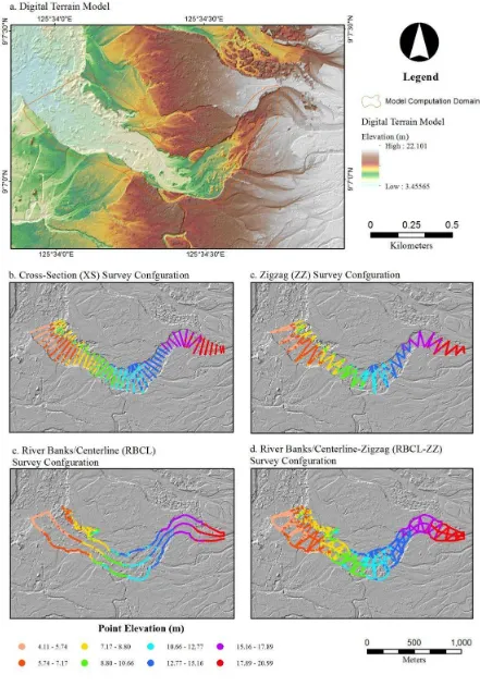
To exemplify how survey configuration and interpolation methods affect the accuracy of river flow simulations, we used a LIDAR DTM of a dried-up portion of Cabadbaran River in Cabadbaran River Basin, Agusan del Norte, Mindanao in Philippines (Figure 1). This portion is approximately 2 km in length, with an average width of 211 m. The dried-up portion of the river is considered to be the true river bed topography. Then, we overlay four (4) types of strategies/configurations (see Figure 1) that are usually implemented when doing river bed elevation surveys. Basically, these configurations define how river bed elevations are to be collected, which can be:
• Along the Cross-sections (XS), at 50-m interval
• As Zig-zag (ZZ), at 100-m interval
• Along the river banks and at the centreline (RBCL)
• Along the river banks and at the centreline with Zig-zag (RBCLZZ)
For the purposes of our investigation, the following procedures are based on the assumption that this portion of the river is submerged with water (e.g., underwater terrain
information is missing in the acquired LiDAR DTM); and that the conduct of surveys is necessary (using the 4 configurations) to generate a river bed topographic surface which will then be integrated into the LiDAR DTM. This bed-integrated DTM will then be used as input to river flow simulation using a 2D hydraulic model.
2.2 River Bed Topography Generation using IDW and Ordinary Kriging
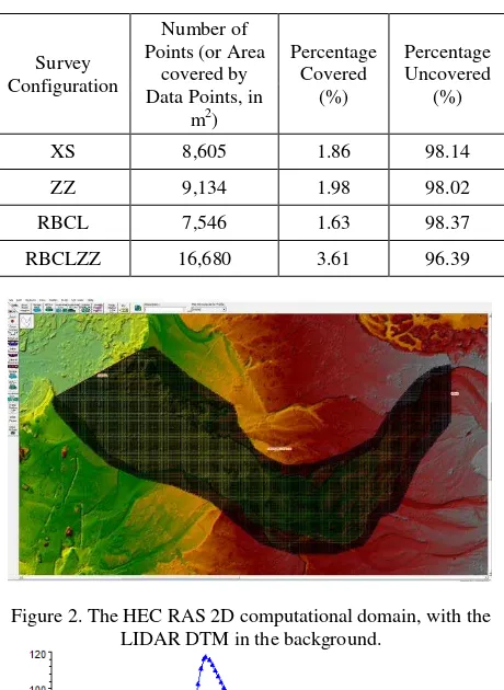
Using ArcGIS 10 software, data points at 1-m interval were generated for each configuration and the true river bed elevation at these points were extracted from the DTM. The data points for each configuration were divided into two sets: 90% were considered as input for interpolation, and the remaining 10% was used for validating the interpolation surface. Table 1 summarizes the number of interpolation data points for each survey configuration, including the percentage coverage of these data points with respect to the surface area of the river bed (462,034 m2), and the area of river bed that was not covered by the data points. It is important to note that each data point uniquely corresponds to a pixel in the DTM, and hence, the area covered by the data points can be obtained by multiplying the number of data points to the area of a pixel which is 1 m2.
We used Inverse Distance Weighting (IDW; n=2) and Ordinary Kriging (OK) to generate the river bed topography for each of the 4 configurations. Numerous trials of IDW and OK interpolations were conducted to find the best parameter values that will produce a 1 m x 1 m resolution river bed surface with the lowest Root Mean Square Error (RMSE). For this purpose, we used the 10% validation points as basis. The interpolated river bed surfaces were then clipped and integrated into the LiDAR DTM using available tools in ArcGIS 10. Overall, a total of 8 bed-integrated DTMs were generated. An independent assessment of the accuracy of the 8 river beds was also conducted using 1,500 random points of known bed elevations. Since these points are unique from those used in all the interpolations, the result of the assessment can be used as bases in determining which of the configurations and interpolation methods are the most superior in terms of accuracy.
2.3 River Flow Simulations Using HEC RAS 2D Hydraulic Model
Table 1. Number of interpolation data points per survey
Figure 2. The HEC RAS 2D computational domain, with the LIDAR DTM in the background.
Figure 3. The inflow boundary condition used in the 2D river flow simulation.
Each of the configured 2D models is then used to simulate the flow of water entering the upstream portion of the river. A 24-hour hydrograph with a peak flow of 123.38 m3/s was utilized as the inflow boundary condition (Figure 3). This hydrograph was computed by a calibrated hydrologic model for this portion. Details about the calibrated model are reported in Santillan and Makinano-Santillan (2015).
To illustrate and quantify how the various interpolated river bed surfaces affect the simulation of river flow, the model domain was set to be initially dry. For the downstream portion, we assigned a “Normal Depth” boundary condition (friction slope = 0.006 based on the average longitudinal slope of the river bed). For a stable model simulation, we set the computational time interval to 10 seconds.
2.4 Accuracy Assessment of the River Flow Simulations
The influence of river elevation survey configuration and interpolation methods was assessed by examining the
maximum flood depth and extent simulated by the 8 2D hydraulic models with different bed-integrated DTMs as inputs. We used as reference in this assessment the maximum flood depth and extent that were simulated by the 2D hydraulic model which utilized the DTM with the true river bed elevations. By comparing each model output, we determined the similarities or differences in maximum flood depth and extent, which we perceived to be related to how the river bed elevation data was “collected” and interpolated. We used the F Measure (Aronica, et al., 2002; Horritt, 2006) to quantify the similarities or differences in the simulated flood extents. The computation was done using the formula:
Where F = the measure of fit
A = the area simulated as “flooded” in both simulations B = the area simulated as “flooded” in the comparison model but simulated as “not flooded” in the reference model (“over prediction”)
C = the area simulated as “not flooded” in the comparison model but simulated as “flooded” in the reference model (“under prediction”)
F = 1 means that the reference and compared flooding extents coincide exactly, while F = 0 means that no overlap exists between the reference and compared flooding extents. Flooding extents generated by the 2D hydraulic model can be assessed either as “Good Fit” (F ≥ 0.7), “Intermediate Fit” (0.7 > F ≥ 0.5), or “Bad Fit” (F < 0.5) (Breilh, et al., 2013).
In addition to the F Measure, we also assessed the differences in maximum flood depth by computing the RMSE of 1,500 points scattered randomly over the model domain.
3. RESULTS AND DISCUSSION
3.1 Interpolated River Bed Surfaces
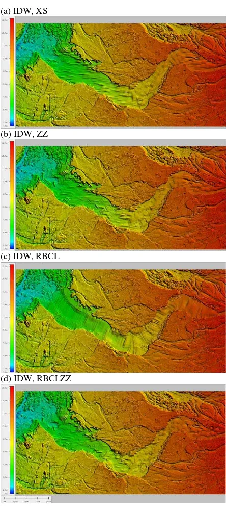
Figures 4 and 5 show the results of the IDW and OK interpolation of the river bed elevation data under various survey configurations. The maps showing the spatial distribution of the differences between the true and interpolated river bed elevations are shown in Figure 6. For the interpolations using the XS configuration, differences in elevation ranges are least pronounced than those interpolations using the RBCL, ZZ and RBCLZZ configurations. The RBCL configuration exhibited the most pronounced differences in elevation values, with many portions having differences ranging from 3 to more than 4 meters.
regardless of the interpolation method used, appears to be the most erroneous among the interpolation results.
(a) IDW, XS
(b) IDW, ZZ
(c) IDW, RBCL
(d) IDW, RBCLZZ
Figure 4. Results of Inverse Distance Weighted (IDW) interpolation.
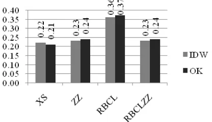
For the XS and ZZ configurations, the use of OK instead of IDW appears to decrease the RMSE values. The reverse is true for the RBCL and RBCLZZ configurations. In both cases, the decrease or increase in RMSE values is very small (0.01 to 0.02 m), and maybe considered insignificant. As such, it can be said that the choice between IDW and OK does not seem to matter as far as the accuracy of the interpolated river bed surfaces is concerned. Using any of the two methods would seem to produce river bed surfaces of similar accuracy.
In the case of survey configurations, two important findings are obvious. The first is that, choosing the RBCL would yield less accurate interpolated surfaces.
(a) OK, XS
(b) OK, ZZ
(c) OK, RBCL
(d) OK, RBCLZZ
Figure 5. Results of Ordinary Kriging (OK) interpolation.
As such, the accuracy of the interpolation (regardless of whether it is IDW or OK) is better compared to the other configurations, especially RBCL, because the number of nearby points that can be used to predict elevations in unmeasured locations are higher.
In the case of ZZ, some large distances between measurements exist, particularly near the river banks/boundaries. For these portions, differences between the interpolated and true elevations were found to occur and contributed to its relatively higher RMSEs compared to XS. In the case of RBCLZZ, while the data coverage seems to have increased, there are still large portions that were left unmeasured. Nevertheless, for both ZZ and RBCLZZ, the unmeasured portions are lesser in area compared to that of RBCL.
The presence of large areas in many portions of the river bed, particularly between the boundary and the center line, that were left unmeasured can be considered the main reason why the interpolated river bed surfaces under the RBCL configuration have larger RMSEs compared to the others. Compared to XS, ZZ or RBCLZZ, the number of nearby points that can be used by the interpolation method in these unmeasured portions is very low, which then led to the erroneous predictions of elevations. The erroneous prediction of elevations in these portions are confirmed by the large differences in elevations as shown in Figure 6, which greatly contributed to the high RMSEs.
All these results highlight the findings by previous researches, particularly those of Heritage et al (2009) and Glenn et al (2016), that the interpolated river bed accuracy is not influenced by the choice of a specific interpolation method but rather by the survey strategy or configuration. The large RMSEs for the RBCL configuration and the low RMSEs for the XS configuration confirm that as the data points become evenly spaced and covers more portions of the river, the resulting interpolated surfaces become more accurate.
3.2 River Flow Simulation Results
Figure 7 shows the maximum flood depths simulated by the 2D hydraulic model using the original DTM (with true river
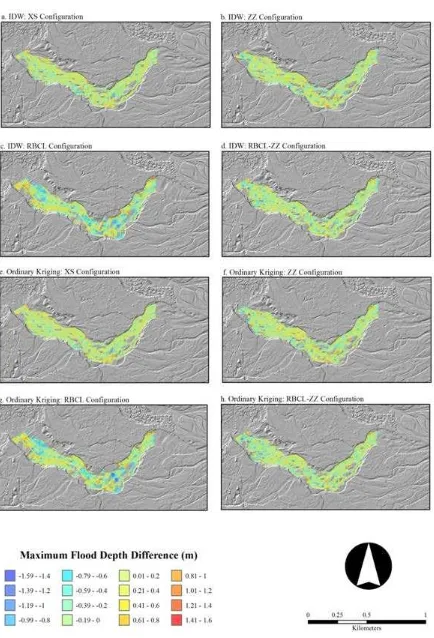
bed elevation) and the 8 DTM integrated with interpolated river bed topography. It can be noticed that none of the 8 results perfectly matched the maximum flood depth and extent that were simulated using the original DTM. This is supported by the differences between the maximum flood depths simulated by the 2D hydraulic model using the original DTM and 8 bed-integrated DTMs (Figure 8).
For the XS configuration, the differences in maximum flood depths are almost uniform while those of the other configurations have large variations. RBCL interpolated surfaces, in particular, exhibited the most pronounced differences in maximum depth values, with many portions having differences ranging from 0.4 to more than 1.5 meters. These large differences can be explained by the presence of erroneous portions of the interpolated river bed surfaces under the RBCL configuration.
Among the 8 results, the XS configuration with OK method was found to give the most accurate maximum flood extent (F=0.84) and maximum flood depth (RMSE=0.21 m) when compared with the extent simulated using the original DTM (Figure 10 and Figure 11). It can be recalled that the interpolated river bed surface resulting from the same configuration and interpolation method was also found to be the most accurate. Furthermore, the levels of accuracy of the river flow simulations for each pair of configuration and interpolation method used linearly corresponds to the levels of accuracy of the interpolated river bed surfaces used in the simulation. If we are to rank the accuracy of the river flow simulations in terms of F and RMSE, XS would be the most accurate, followed by RBCLZZ, ZZ and RBCL. The same ranking can be said in terms of river bed surface accuracy. This finding proves that accurate river bed information will also result to accurate river flow simulation as far as the maximum flood depth and extent are concerned.
Figure 8. Difference in maximum flood depths simulated by the 2D hydraulic model using the original DTM and 8 bed-integrated DTMs. A negative difference means the maximum flood depth simulated by the model using a DTM with interpolated river bed is
Figure 9. Root Mean Square Error (RMSE) of the interpolated river bed surfaces using an independent set of
1,500 random points.
Figure 10. F values of the simulated maximum flood extent.
Figure 11. RMSE of simulated maximum flood depths.
4. SUMMARY AND CONCLUSIONS
In this work, we investigated how survey configuration and the type of interpolation method can affect the accuracy of river flow simulations that utilize LIDAR DTM integrated with interpolated river bed as its main source of topographic information. Aside from determining the accuracy of the individually-generated river bed topographies, we also assessed the overall accuracy of the river flow simulations in terms of maximum flood depth and extent. Four survey configurations consisting of river bed elevation data points arranged as cross-section (XS), zig-zag (ZZ), river banks-centerline (RBCL), and river banks-banks-centerline-zig-zag (RBCLZZ), and two interpolation methods (IDW and OK) were considered.
The major conclusion that we can draw from this work is that the choice of survey configuration, rather than the interpolation method, has significant effect on the accuracy of the interpolated river bed surfaces, and subsequently on river flow simulations. The RMSEs of the interpolated surfaces and the model results vary from one configuration to another, and depends on how each configuration evenly collects river bed elevation data points. The large RMSEs for the RBCL configuration and the low RMSEs for the XS configuration confirm that as the data points become evenly spaced and covers more portions of the river, the resulting interpolated surface and the river flow simulation where it was used also become more accurate.
The XS configuration with OK as interpolation method provided the best river bed interpolation and river flow simulation results. The RBCL configuration, regardless of the interpolation method used, resulted to least accurate river bed surfaces and simulation results. Based on the accuracy statistics obtained, the use of XS configuration to collect river bed data points and applying the OK method to interpolate the river bed topography are the best methods to use to produce satisfactory river flow simulation outputs. The use of other configurations (and a choice between IDW or OK) except RBCL can also be an alternative in cases when the XS configuration is less practical or expensive to implement.
All these findings and conclusions, however, are limited only to the survey configurations and interpolation methods, including the river flow simulation approach used. While this work was able to show the effects of survey configuration and interpolation methods on the accuracy of LIDAR DTM-based river flow simulations, it has a number of limitations. Firstly, the study area was only confined to a short portion (~ 2 km) of a relatively straight river. The results may be different if the analysis is to be conducted in a rather long or meandering river.
Secondly, the suitability of the flow data used in the simulation was not checked. For this work, the input flow data did not led to a condition where the river overflows. Using flow data of higher magnitudes than the one used here may result to different F and RMSE values. Another limitation is the use of a 5 m x 5 m mesh during the simulation. This inevitably has degraded river bed topographic information such that the maximum flood depths and extents that were generated by the model using this mesh size may vary from those generated using a 1 m x 1 m mesh.
ACKNOWLEDGEMENTS
REFERENCES
Aronica, G., Bates, P. D., Horritt, M. S., 2002. Assessing the uncertainty in distributed model predictions using observed binary pattern information within GLUE. Hydrological Processes, 16(10), pp. 2001-2016.
Breilh, J. F., Chaumillon, E., Bertin, X., Gravelle, M., 2013. Assessment of static flood modeling techniques: application to contrasting marshes flooded during Xynthia (western France). Natural Hazards and Earth System Science, 13(6), pp. 1595-1612.
Caviedes-Voullième, D., Morales-Hernández, M., López-Marijuan, I., García-Navarro, P., 2014. Reconstruction of 2D river beds by appropriate interpolation of 1D cross-sectional information for flood simulation. Environmental Modelling & Software, 61, pp. 206-228.
Conner, J. T., Tonina, D., 2014. Effect of cross-section interpolated bathymetry on 2D hydrodynamic model results in a large river. Earth Surface Processes and Landforms, 39, pp. 463-464.
Cook, A., Merwade V., 2009. Effect of topographic data, geometric configuration and modeling approach on flood inundation mapping. Journal of Hydrology, 377, pp. 131– 142.
Glenn, J., Tonina, D., Morehead, M. D., Fiedler, F., Benjankar, R., 2016. Effect of transect location, transect spacing and interpolation methods on river bathymetry accuracy. Earth Surfaces Processes and Landforms, 41, pp. 1185–1198.
Goff, J.A., Nordfjord, S., 2004. Interpolation of fluvial morphology using channel oriented coordinate transformation: a case study from the New Jersey shelf. Mathematical Geology, 36 (6), pp. 643–658.
Heritage, G. L., Milan, D. J., Large, A. R., Fuller, I. C., 2009. Influence of survey strategy and interpolation model on DEM quality. Geomorphology, 112(3), pp. 334-344.
Hilldale, R. C., Raff, D., 2008. Assessing the ability of airborne LiDAR to map river bathymetry. Earth Surface Processes and Landforms, 33(5), pp. 773-783.
Horritt, M. S., 2006. A methodology for the validation of uncertain flood inundation models. Journal of Hydrology, 326, pp. 153-165.
Legleiter, C. J., Kyriakidis, P. C., 2008. Spatial prediction of river channel topography by kriging. Earth Surface Processes and Landforms, 33, pp. 841–867.
Mandlburger, G., Hauer, C., Höfle, B., Habersack, H., Pfeifer, N., 2009. Optimisation of LiDAR derived terrain models for river flow modelling. Hydrology and Earth System Sciences, 13(8), pp. 1453-1466.
Merwade, V., Cook, A., Coorod, J., 2008. GIS techniques for creating terrain models for hydrodynamic modeling and flood inundation mapping. Environmental Modelling & Software, 23, pp. 1300-1311.
Merwade, V., 2009. Effect of spatial trends on interpolation of river bathymetry. Journal of Hydrology, 371(1), pp. 169-181.
Merwade, V. M., Maidment, D. R., Goff, J. A., 2006. Anisotropic considerations while interpolating river channel bathymetry. Journal of Hydrology, 331(3), pp. 731-741.
Santillan, J. R., Makinano-Santillan, M., 2015. Analyzing the impacts of tropical storm-induced flooding through numerical model simulations and geospatial data analysis. In: 36th Asian Conference on Remote Sensing 2015, Quezon City, Philippines.
Schappi, B., Perona, P., Schneider, P., Burlando, P., 2009. Integrating river cross section measurements with digital terrain models for improved flow modelling applications. Computers and Geosciences, 36, pp. 713-716.
Turner, A. B., Colby, J. D., Csontos, R. M., Batten, M., 2013. Flood modeling using a synthesis of multi-platform LiDAR data. Water, 5(4), pp. 1533-1560.