A Comparison between Normal and Non-Normal Data in Bootstrap.

(1)

A Comparison between Normal and Non-Normal

Data in Bootstrap

Suliadi Firdaus Sufahani

Department of Science and Mathematics,

Faculty of Science, Technology and Human Development, Universiti Tun Hussein Onn Malaysia, Parit Raja,

86400 Batu Pahat, Johor, Malaysia

Asmala Ahmad

Department of Industrial Computing,

Faculty of Information and Communication Technology, Universiti Teknikal Malaysia Melaka,

Hang Tuah Jaya, 76100 Durian Tunggal, Melaka, Malaysia

asmala@utem.edu.my

Abstract

In the area of statistics, bootstrapping is a general modern approach to resampling methods. Bootstrapping is a way of estimating an estimator such as a variance when sampling from a certain distribution. The approximating distribution is based on the observed data. A set of observations is a population of independent and observed data identically distributed by resampling; the set is random with replacement equal in size to that of the observed data. The study starts with an introduction to bootstrap and its procedure and resampling. In this study, we look at the basic usage of bootstrap in statistics by employing R. The study discusses the bootstrap mean and median. Then there will follow a discussion of the comparison between normal and non-normal data in bootstrap. The study ends with a discussion and presents the advantages and disadvantages of bootstraps.

(2)

1 Introduction

Bootstrap is well known as a resampling procedure. Resampling starts with

drawing a sample from the population. For example, x = (x1, x2,…xn) is a sample. Then from the sample another sample, X*= (X1*, X2*,…Xn*), is drawn

randomly with replacement. This technique is called resampling. Resampling, in other words, draws repeated samples from the given data. Bootstrapping and permutation are mostly used in statistics. Resampling is now widely used for confidence limits, hypothesis tests and other inferential problems. Resampling lets us analyse the sorts of data, even data with complex structures, for example regression models. However, which residuals should be resampled? This is one of the most confusing questions that arise in terms of regression prospects. Therefore, raw residuals leave one option and another one is studentized residuals, which are mostly involved in linear regressions. By using the studentized residual, it will make it easy for us to compare and run the results and it will not give us a major difference in actual practice.

2 Bootstrap Methods

Let us consider a certain situation with a common data, where a random sample x = (x1,x2,…xn) from an unknown distribution F has been observed. Then we try

(3)

technique, such as the t-test and F-test.

Fig. 1. Schematic of the bootstrap process for estimating the standard error of a statistic [1].

3 Comparison of Resampling Methods

Table 1 shows a comparison of the methods for testing the equality means of two populations [4].

Table 1: Comparison of resampling methods.

Permutation Rank (Wilcoxon) Nonparametric Bootstrap

Parametric (t-test)

Choose test statistic Choose test statistic Choose test statistic Choose the test statistic whose distribution can be derived

Calculate statistic Convert to ranks Calculate statistic

(4)

4 Mean Bootstrap

There are several methods for a single parameter and in our case we are considering the mean bootstrap. The methods are the percentile method,

Lunneborg’s method, traditional confidence limits and bootstrapped t intervals. The mean bootstrap is the simplest out of the bootstrapping procedures and the result will appear straightforward. In fact, it produces very nice confidence intervals on the mean and it is more sensible if we understand the mean in terms of statistics. Based on [1] along with a number of other researchers, he has come up with better limits. We develop an example for this case in order to explain this better. Firstly, we construct a set of data consisting of 50 random normal data and apply it to a simple linear regression [3]. Then we calculate the confidence interval for the data. The result is shown in Table 2.

Table 2: (a) Results from the example and (b) 90 % confidence interval for the mean statistic.

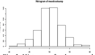
Figure 2 shows the results of generating 95% confidence limits on the mean. The lower limit is 45.3755 units below the mean, while the upper is 54.704 units above the mean. We can also see that the distribution of the means is approximately normal, and the standard error of this bootstrapped distribution with its standard error is 2.802816.

Fig. 2. Histogram for the example.

5 Median Bootstrap

The same thing goes for the median bootstrap; it uses the same method as the

mean bootstrap, which is the percentile method, Lunneborg’s method, traditional

(5)

confidence limits or bootstrapped t intervals. We will not repeat this here; the result should be as straightforward as that for the mean bootstrap. We develop our own example for the case in order to better explain how to involve the median in bootstrapping. Firstly, we generate random data (for example, normal) and we use it as our raw data for the simple bootstrap and in this case we use 10 normal random data entries as our original data. Then we find the mean and the standard deviation of the original data. From the original data, we generate bootstrap samples by taking a certain amount (such as 20 in this example) of observations with 100 replications for each bootstrap sample with the mean and standard deviation. The mean of the data is considered to be the normal mean because it comes from a normal distribution of the data set. Then we calculate the median and standard error for each bootstrap and compare the original data with the resampling. As mentioned, we create a set of data consisting of 10 normal random data entries as shown in the table below. With a further calculation, we obtain a normal mean of 4.6 and the standard deviation is 2.875181 (Table 3).

Table 3: (a) Result from the set of normal random data and (b) mean and standard deviation.

(a)

Random

Data 1 2 3 4 5 6 7 8 9 10

(b)

Mean Standard Deviation

4.6 2.875181

(6)

Table 4: 100 replications for the first bootstrap sample out of 20 bootstrap samples.

5 6 4 2 6 6 4 4 5 4

-1 6 5 1 6 3 0 3 7 6

0 5 2 7 2 8 5 5 6 7

6 0 10 1 6 0 4 8 5 4

4 7 7 3 4 5 6 3 2 0

4 4 7 4 6 2 5 5 0 7

8 1 5 5 7 3 6 4 2 5

7 5 11 6 6 4 5 3 3 4

7 5 2 1 8 6 5 6 4 4

8 0 4 8 6 1 6 1 6 5

Then we calculate the median for each bootstrap sample as shown in Table 5. Once we obtain the median for each bootstrap sample, we continue with the next procedure, which is calculating the standard deviation of the bootstrap distribution. Based on the resample median, we can find the standard deviation.

Table 5: (a) Median for all the 20 bootstrap samples that we generate and (b) the standard deviation.

(a)

1 2 3 4 5 6 7 8 9 10

4 4.5 4 5 4 5 5 5 5 4

11 12 13 14 15 16 17 18 19 20

5 5 5 5 5 4 5 5 6 5

(b)

Standard Deviation 0.2236068

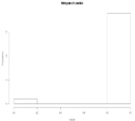
In order to see the bootstrap median, we construct a histogram for the distribution of the medians (Figure 3).

Fig. 3. Distribution bootstrap median based on the study.

(7)

rather than the value of 4. Furthermore, the standard deviation of the bootstrap sample is 0.2236068. For further studies, we can put all these steps into a single function where all we would need to do is to specify the data set and how many times we want to resample in order to obtain the adjusted standard error of the median.

6 Monte Carlo Looping With Bootstrap In A Simple Linear Case

For Normal And Non-Normal Data

An exploratory analysis of the summary statistics for the response variables and explanatory variables is carried out to calculate the simple regression case for the normal and non-normal data in bootstrap. To make the interpretation easy, a few graphical representations using a histogram are also carried out at the end of each result. Before going for statistical modelling, the correlations between response and explanatory variables are examined by illustrating a few scatter plots. The data given is already in a linear relationship between the response and explanatory variables. An exploratory analysis of the data is carried out using the R statistical tool. We are dealing with a simple linear regression. For a simple regression the statistical model can be expressed as follows:

yi= β0 + β1xi + ei, ei~ N(0,σ2e) (1)

where yiis the response of interest, β0 is the overall mean, xi is the independent

variable and ei is the normally distributed residual term. For the estimation

coverage of the bootstrap and classical methods, we perform the correlation model in the simple linear regression to obtain the property of beta-one (β1), where β1 is

the slope. However, we are using Monte Carlo looping 100 times. The result will indicate the true value of the parameter in the classical method and bootstrap method. Then we calculate the estimation coverage of the confidence interval and the general formula is shown below:

m

1

Estimation Coverage of CI I

M

 

  _{ }



(2)

M = number of times there is Monte Carlo looping

m

I



= the sum of times when the fixed value of β1 lies within the lower and

upper bounds or, in other words, it contains a true parameter.The estimation coverage is carried out for the normal and non-normal data and from there we compare the differences between the two distributions, using the bootstrap and classical methods. In this example, firstly, we fix up the value of beta-one (β1)

(8)

or non-normal, such as gamma) with a mean of 100 and a standard deviation of 50 as our original data for independent variables (x) and another 100 normal random data entries with a normal mean of 0 and a standard deviation of 50 for dependent variables (y). In this example, y is the dependent variable and x is the independent variable. We set the calculation by generating 200 bootstrap samples where each sample is observed with 100 replications. From there we find the 95% confidence interval for the mean statistics for the classical method and the bootstrap method. Then we calculate the estimation coverage by checking whether the fixed value of

β1 lies within the lower and upper bounds for the bootstrap and classical methods.

As mentioned earlier, we give the value of 1 when it lies and 0 otherwise

6.1 Normal Data

Firstly, we fixed the value of beta-one (β1) as 0.3 from the population. Therefore,

the equation is as follows:

yi= β0 + 0.3xi + ei, ei~ N(0,σ2e) (3)

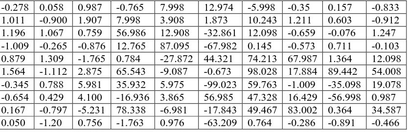
Secondly, we set up a sample data set, which is the independent variable (x) with normal random data. The sample set consists of 100 data entries for x and we want to use the mean top to describe the centre of the data. We run Monte Carlo looping 200 times; so there are 200 sample sets with a different data set for every loop. The data in Table 6 is one of the sample sets out of 200 sets.

Table 6: One of the examples of the data set for x.

-0.278 0.058 0.987 -0.765 7.998 12.974 -5.998 -0.35 0.157 -0.833

1.011 -0.900 1.907 7.998 3.908 1.873 10.243 1.211 0.603 -0.912

1.196 1.067 0.759 56.986 12.908 -32.861 12.098 -0.659 -0.076 1.247

-1.009 -0.265 -0.876 12.765 87.095 -67.982 0.145 -0.573 0.711 -0.103

0.879 1.309 -1.765 0.784 -27.872 44.321 74.213 67.987 1.364 12.098

1.564 -1.112 2.875 65.543 -9.087 -0.673 98.028 17.884 89.442 54.008

-0.345 0.788 5.981 35.932 5.975 -99.023 59.763 -1.009 -35.098 19.078

-0.654 0.429 4.100 -16.936 3.865 56.985 47.328 16.429 -56.998 0.987

0.167 -0.797 -5.231 78.338 -6.981 -17.843 49.467 83.002 0.364 34.587

0.050 -1.20 0.756 -1.763 0.976 -63.209 0.764 -0.286 -0.891 -0.466

(9)

Table 7: One of the examples of the set of data for y.

73.586 105.603 66.304 114.935 20.785 196.067 215.079 157.364 13.353 213.675

201.366 37.3447 57.017 171.174 125.463 125.616 133.205 194.818 173.922 247.951

92.717 112.443 152.764 72.760 66.644 219.722 186.013 8.291 209.785 192.843

79.576 185.700 94.843 93.094 171.878 70.877 141.636 45.366 173.922 117.795

15.268 -14.105 135.989 218.542 70.877 70.877 72.959 284.018 53.288 142.644

15.268 91.355 111.646 129.773 4.120 195.769 45.535 -25.517 53.288 142.644

26.449 76.382 215.630 156.986 106.170 65.775 99.969 4.955 -19.497 127.430

-59.724 192.107 50.378 74.778 106.170 168.468 167.576 153.017 113.437 287.776

90.200 104.754 112.492 64.250 239.187 23.818 131.103 109.365 -34.964 -18.050

-49.795 120.135 -10.081 -53.994 321.957 214.047 201.541 117.073 247.951 174.954

From the data above, as mentioned earlier, we determine that x is an independent variable and y is a dependent variable. The study continues by generating 200 bootstrap samples for both x and y and each bootstrap sample has 100 replications, with a significant level of 5%. In this section, we perform the correlation model in

the simple linear regression and obtain the property of β1, where β1 is the slope.

However, we are using Monte Carlo looping 200 times. The results are indicated using the classical method and bootstrap methods. The results below show an example of the lower and upper bounds of β1 for the first set out of the 200 sets.

Table 8 shows that, by using the classical method, we set up a calculation to indicate whether the fixed value of β1 lies between the lower and upper bounds for

the classical method and bootstrap methods.

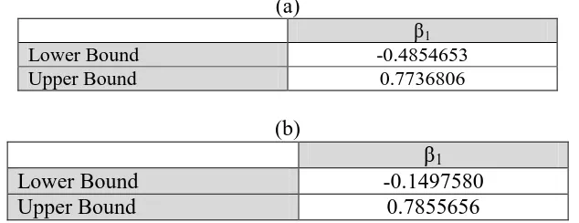
Table 8: One of the examples of the lower and upper bounds for the 95% confidence interval using (a) the classical method and (b) the bootstrap method.

(a)

β1

Lower Bound -0.4854653

Upper Bound 0.7736806

(b)

β1

We have run the Monte Carlo looping 200 times and from the simulation, in 198

out of 200 times, the fixed value of β1 lies between the lower and upper bounds

for the classical method and, in 187 out of 200 times, the fixed value of β1 lies

(10)

For the classical method,

m

1 1

Estimation Coverage of CI I *198 0.96

M 200

   

_{ } _ _ 

 



  (5)

From the results, if we fix the value of the β1, which is 0.3, we can see that the

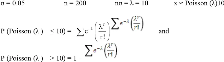
classical method covers 96% of the fixed value within it lower and upper bounds and the bootstrap method covers 93.5% of the fixed value within its lower and upper bounds. It seems that, for normal cases, both the classical method and the bootstrap method have a value for the estimation coverage that is nearly the same as that for the 95% confidence interval. This is true if we base this on the rules below (for example, the Poisson distribution):

α = 0.05 n = 200 nα = λ = 10 x ≈ Poisson (λ)10 value of the percentage of the confidence interval. Then a further study is carried out by changing the value of the fixed β1 (Table 9).

Table 9: Future test of the estimation coverage by changing β1 value.

(11)

6.2 Non-Normal Data (Gamma-Distribution)

Firstly, we fix the value of β1 at 0.3 for the population. Therefore, the equation is

as follows:

yi= β0 + 0.3xi + ei X~Gamma (k,θ) (6)

As we know, the pdf for the gamma distribution is:

 

where a is the shape and s is the scale. Therefore, the mean and variance for the gamma distribution are E(X) = a*s and Var(X) = a*s2. In this study we set the value of the mean as 10 and the value of variance as 20. Secondly, we set up sample data set with the independent variable (x) and non-normal random data. The sample set consists of 100 data entries for x and we want to use the mean top to describe the centre of the data. We run Monte Carlo looping 200 times, so there will be 200 sample sets with a data set with every loop. The data in Table 10 is for one of the sample sets out of 200 sets.

Table 10: One of the examples of the data sets for x.

11 4 6 15 21 23 16 9 18 5

(12)

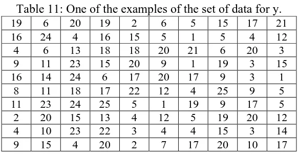
Table 11: One of the examples of the set of data for y.

19 6 20 19 2 6 5 15 17 21

16 24 4 16 15 5 1 5 4 12

4 6 13 18 18 20 21 6 20 3

9 11 23 15 20 9 1 19 3 15

16 14 24 6 17 20 17 9 3 1

8 11 18 17 22 12 4 25 9 5

11 23 24 25 5 1 19 9 17 5

2 20 15 13 4 12 5 19 20 12

4 10 23 22 3 4 4 15 3 14

9 15 4 20 2 7 17 20 10 17

From the data above, as mentioned earlier, we determine that x is an independent variable and y is a dependent variable. The study continues by generating 200 bootstrap samples for both x and y and each bootstrap sample has 100 replications, with a significance level of 5%. In this section, we perform the correlation model in a simple linear regression and obtain the property of β1, where β1 is the slope.

However, we are using Monte Carlo looping 200 times. The results are indicated for the classical method and bootstrap methods. The results in Table 12 shows an example of the lower and upper bounds of β1 for the first set out of 200 sets.

Table 12: One of the examples of the lower and upper bounds for the 95% confidence interval using (a) the classical method and (b) the bootstrap method.

(a)

β1

(b)

β1

Based on the table above, we set up a calculation to indicate whether the fixed value of β1 lies between the lower and upper bounds for the classical method and

bootstrap method. We run the Monte Carlo looping 200 times and from the simulation, in 189 out of the 200 times, the fixed value of β1 lies between the

lower and upper bounds for the classical method and, in 181 out of 200 times, the fixed value of β1 lies between the lower and upper bounds for the bootstrap

(13)

For the classical method,

m

1 1

M 200

M 200 However, the bootstrap method covers 90.5% of the fixed value in its lower and upper bounds. It seems that, for non-normal cases, the classical method has a high range of lower and upper bounds when compared to the bootstrap method. It seems that, for normal cases, both the classical method and bootstrap method have a value for the estimation coverage that is nearly the same as that for 95% of the confidence interval even though we are dealing with non-normal data, which is the gamma distribution. This is true if we base this on the rules below, which is the same as for our discussion of the earlier results (for example, the Poisson distribution), which is the same as we discussed earlier in the normal data section. Based on the rule, the value of the estimation coverage should be close to the value of the percentage of the confidence interval. Then we carry out a further study by changing the value of the scale (s) and shape (a) in order to see the estimation coverage for each method (Table 13).

Table 13: Future test of the estimation coverage by changing the value of the shape (a) and scale (s).

(14)

7 Conclusion and Discussion

Based on the study, a general explanation has been given regarding the background to bootstrap. All the procedures of bootstrap have been discussed to provide further understanding of the application of bootstrap as well as a simple calculation for bootstrapping using R. An analysis of the data has been conducted in order to find the mean and median for bootstrap. From the results we can see that bootstrap gives a better result than the original value if we compare both results. Furthermore, the authors are using the Monte Carlo technique and looping. From there we say can that, whether we are using normal or non-normal data, both the estimation coverage for bootstrap and the estimation coverage for the classical method are close to the value of the confidence interval. Furthermore, if we use non-normal data, at the end of bootstrapping we can see that the distribution appears to be nearly normal. In the future, we should consider using bootstrapping in the Monte Carlo technique and looping in the Bayesian diagnostic or time series. From there we can see the pattern of the distribution and the implementation of the results. The study should be conducted on both normal and non-normal data. The advantage of bootstrapping is that the result is simple and straightforward even when it involves a complex parameter. However, the disadvantage is that it does not provide a sample guarantee and has a tendency to make certain important assumptions, such as the independence of a sample.

References

[1] B. Efron, R. Tibshirani, An Introduction to the Bootstrap, Chapman & Hall/CRC, Florida, 1993.

[2] G. David, Bootstrapping and the Problem of Testing Quantitative Theoretical Hypothesis, Middle East Technical University, 2002.

[3] J. Fox, Bootstrapping Regression Model, Brown University, 2002.

[4] P. Good, Permutation Test, 2nd ed, Springer, New York, 2000.

[5] P. Good, Resampling Method, 3rd ed, Birkhauser, Boston, 2006.