Statistical Analysis for Non-Normal and Correlated Outcome in Panel Data

STATISTICAL ANALYSIS FOR NON-NORMAL

AND CORRELATED OUTCOME IN PANEL DATA

ANNISA GHINA NAFSI RUSDI

DEPARTMENT OF STATISTICS

FACULTY OF MATHEMATICS AND NATURAL SCIENCES INSTITUT PERTANIAN BOGOR

THE BACHELOR THESIS STATEMENT AND SOURCES OF

INFORMATION AND COPYRIGHT DEVOLUTION

I hereby declare that the bachelor thesis entitled Statistical Analysis for Non-Normal and Correlated Outcome in Panel Data is my work under the guidance of the supervisory committee and it has not been submitted in any form to any college. Resources derived or quoted from works published and unpublished from other writers are mentioned in the text and listed in the Bibliography at the end of this bachelor thesis.

I hereby bestow the copyright of my papers to the Bogor Agricultural University.

Bogor, October 2014

Annisa Ghina Nafsi Rusdi

ABSTRACT

ANNISA GHINA NAFSI RUSDI. Statistical Analysis for Non-Normal and Correlated Outcome in Panel Data. Supervised by ASEP SAEFUDDIN and ANANG KURNIA.

There are many cases that cannot fulfill some assumptions in statistical analysis, such as normality and independence. In many practical problems, the normality as well independent assumption is not reasonable. For example, data that repeated over time tend to be correlated. If analysis ignores the non independent outcome the Standard Error (SE) on the parameter estimates tends to be too small. Generalized Linear Model (GLM), Generalized Estimating Equation (GEE), and Generalized Linear Mixed Model (GLMM) can be used for non-normal data using the link functions. GEE includes working correlation matrix to accommodate the correlation in the data. GLMM may overcome the repeated observation and allows individual have different baseline/intercept. The study is aim at comparing result based on those approaches. The data that are used in this study are from BPS and the outcome that are used is poverty proportion. Based on the study shows that GEE approach is better than GLM for marginal model, and GLMM approach is better than GEE with dummy variable.

A Bachelor Thesis

in partial fulfillment of the requirements for the degree of bachelor of statistics

in

Department of Statistics

STATISTICAL ANALYSIS FOR NON-NORMAL

AND CORRELATED OUTCOME IN PANEL DATA

DEPARTMENT OF STATISTICS

FACULTY OF MATHEMATICS AND NATURAL SCIENCES INSTITUT PERTANIAN BOGOR

BOGOR 2014

Title : Statistical Analysis for Non-Normal and Correlated Outcome in Panel Data

Name : Annisa Ghina Nafsi Rusdi

NIM : G14100069

Approved by

Prof Dr Ir Asep Saefuddin, MSc Advisor I

Dr Anang Kurnia, MSi Advisor II

Acknowledged by

Dr Anang Kurnia, Msi Head of Department

PREFACE

All best praise and regards to llah Subhanahu Wata’ala. Because of Allah, this research and bachelor thesis could be done. This research theme is about non-normal and correlated outcome with the title is Statistical Analysis for Non-Normal and Correlated Outcome in Panel Data and it is conducted from February 2014 until September 2014.

Thank you Prof Asep Saefuddin and Dr Anang Kurnia as the advisors of this research. Also big thanks for both of my dearest parents (ayah ibu, I love you), my dearest sister (ade, you are the best partner in my life), my roommate Ka Husnul Puncul, statistika 47, all of the staff in Department of Statistics, Sakinah Gang (you are the best), AgCN (ma pal, you all guys are so cool), and all of my friends, your support has always been my spirit and encouragement. I hope this research will give benefit for academics.

Bogor, October 2014

TABLE OF CONTENTS

TABLE LIST vi

TABLE OF FIGURE vi

TABLE OF APPENDIX vi

INTRODUCTION 1

Background 1

Objective of The Study 2

DATA AND METHODOLOGY 2

Data Source 2

Methodology 2

RESULT 6

Exploration of the Data 6

GLM Approach 6

GEE Approach 7

GLMM Approach 8

GEE Approach with Dummy Variable 9

Model Comparison 9

CONCLUSION 10

REFERENCES 10

APPENDIX 11

TABLE LIST

1. Example of the link function 3

2. Common working correlation matrix 4

3. Parameter estimates and standard errors (GLM approach) 7 4. Parameter estimates and standard errors (GEE approach) 8

TABLE OF FIGURE

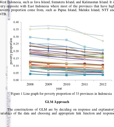
1. Line graph for poverty proportion of 33 provinces in Indonesia 6

TABLE OF APPENDIX

1. Parameter estimates and standard errors (GLMM approach) 11 2. Parameter estimates and standard errors (GEE approach with dummy

variable) 12

INTRODUCTION

Background

Methods of statistical analysis depend on the measurement scales of the response and explanatory variables. In many practical problems, the normality assumption is not reasonable. In some cases the response variable can be transformed to improve linearity and homogeneity of variance. But this approach has some drawbacks such as response variable has changed (not original) and transformation must simultaneously improve linearity and homogeneity of variance.

Panel analysis combines the time series and cross-sectional data. Models that usually used in panel analysis are Pooled Model, Fixed Effects Model, and Random Effects Model. The outcome that are used in this study is not normal and correlated.

Data that repeated over time tend to be correlated or dependent each other. Individuals tend to be more similar to themselves over time than the other independent individuals. Group of individuals may have dependent outcome. The Standard Error (SE) of the estimate is very small in the case of ignore dependent outcome.

If the assumptions are violated, such as response variable is not normally distributed and correlated, the classic model like Panel Regression may produce missleading conclusion. There are some approaches for this kind of data (non-normal and correlated outcome). Pooled Model is approached by Generalized Linear Model (GLM) and Generalized Estimating Equation (GEE), Fixed Effects Model is approached by Generalized Estimating Equation with dummy variable, and Random Effects Model is approached by Generalized Linear Mixed Model (GLMM).

GLM can solve the problem of non-normal data distributed. GLM introduced by Nelder and Wedderburn (1972) are standard method used to fit regression model for univariate data that are presumed to follow an exponential family distribution (Horton and Lipsitz 1999). It is possible to fit models of data from normal, inverse Gaussian, gamma, Poisson, binomial, geometric, and negative binomial by suitable choice of the link function g(.).

GEE can solve the problem of non-normal and correlated data. Liang and Zeger (1986) introduced GEE to take into account correlation between observations in GLM. GEE takes into account the dependency of observation by specifying a “working correlation matrix”. The working correlation matrix is not usually known and must be estimated.

GLMM is a little bit different than GLM and GEE. It has random effect where you can have different intercept for every observation if you assume that the intercept of each observation is different.

2 Domestic Regional Product per Capita by province (Rp10.000) (GDRPC).

Methodology

The procedures of data analysis implemented are: 1. Exploration of the data

Make a plot for the outcome (poverty) to obtaine information on province with the highest and lowest poverty.

Data structure (Dobson 2002):

Panel regression that are usually used (Gujarati 2004):

3

 Fixed Effects Model: y x_iβ _{i it} ; where _i

 Random Effects Model: y x_iβ _{i it} ; where _i . 2. Applying Generalized Linear Model (GLM)

GLM model for independent data are characterized by: g i g _i xi β

where _{i i} , g is a link function. Some examples of the link function can be seen in Table 1.

Response variable which is assumed to share the same distribution from exponential family. The values of the β coefficients are obtained by maximum likelihood estimation. The maximum likelihood estimator of the p x parameter vector β is obtained by solving estimating equation forβ.

_i

Vi is vector of variance, and assuming that responses for different subjects are independent, where O denotes a matrix of zero, (Dobson 2002).

Hence the GLM model for binomial distribution using logit link function was expressed as the following:

log i

- _i β β β U β . 3. Applying Generalized Estimating Equation (GEE)

GEE is a method of estimation of regression model parameters when dealing with dependent data and extension of Generalized Linear Model (GLM) for

4

longitudinal data analysis using quasi-likelihood estimation. When data are collected on the same units across in time, these repeated observations are dependent over times. If this dependent is not taken into account then the Standard Error (SE) of the parameter estimates will not be valid and hypothesis testing result will be non-replicable.

GEE model for correlated outcome is the same as GLM: g i g _i xi β

GEE accommodated correlated outcome using Working Correlation Matrix. GEE includes a working correlation matrix in the SE calculation.

Working variance-covariance matrix for equals:

where is n x n diagonal matrix with elements var(y_ik), _iis n x n “working” correlation matrix for y_i, is a constant to allow for over dispersion.

G estimator of β is the solution of:

Table 2 Common working correlation matrix

5 4. Applying Generalized Linear Mixed Model (GLMM)

Subject-specific models assume that every region has its own intercept. To avoid correlation away regions, each province is assumed to have its own model. The GLMM of subject-specific models rope with this condition. GLMM model for binomial distribution using logit link function with random intercept was expressed as the following:

g i g _i xiβ vi

where v_i is the random effect (one of each subject). These random effect represent the influence of subject i on repeated subjects that is not captured by observed covariates.

The mixed model equations are (Henderson 1984)

βv

_{y y}

GLMM model for this study is: log i An extension of the R2 measure is calculating using:

6

This measure is interpreted as the proportion of variance in the outcome that is explained by the model (Hardin and Hilbe 2003).

RESULT

Exploration of the Data

The poverty proportion of 33 provinces in Indonesia can be seen in Figure 1, shows that the poverty proportion of 33 provinces are random. As we can see in Figure 1, the poverty proportions for most of provinces are decreasing every year. As we can see in Figure 1, the provinces that have high poverty proportion are Papua, Papua Barat, Maluku, Nusa Tenggara Timur (NTT), Nusa Tenggara Barat (NTB), Nangro Aceh Darussalan (NAD), Lampung, Sulawesi Tengah, Bengkulu, and Sulawesi Tenggara. The provinces that have low poverty proportion are Jakarta, Bali, Kalimantan Selatan, Banten, Kalimantan Tengah, Kepulauan Bangka Belitung, Kalimatan Timur, Kepulauan Riau, Jambi, Sulawesi Utara. The rest provinces are in the middle class.

The provinces that have the low poverty proportion are commonly from West Indonesia, such as Java Island, Sumatera Island, and Kalimantan Island. It is very opposite with East Indonesia where most of the provinces that have high poverty proportion come from, such as Papua Island, Maluku Island, NTT and NTB.

7 probability distribution. Because the response variable in the data is proportion so the probability distribution for the response variable is binomial with log i

- _i as the link function.

The parameters estimate and Standard Errors (SEs) for GLM approach can be seen in Table 3.

The model estimation for GLM approach in this study is: log i

i . . . U .

and for GLM approach is 31.1569%. It is interpreted as the 31.1569% proportion of variance in the outcome that is explained by the model.

Scatter plot between prediction values and residual in Appendix 3 shows that residual scale are still large, that are from -0.12 until 0.23. It is bacause the approach that used is not enough to explain the data and it is in accordance with the from GLM approach that is only 31.1569%.

GEE Approach

The construction of GEE is by deciding the working correlation matrix that we will use. In this study, working correlation matrix that was used is autoregressive (AR(1)). The reason for using AR working correlation matrix is measurement closer in time are likely to be more correlated than measurement further apart in time.

Working correlation matrix (AR(1)) for this approach is: . . . . .

Table 3 Parameters estimate and standard errors (GLM approach) Parameter Estimate Standard Error

Intercept 3.7367 0.0030

HDI -0.0708 0.0000

UR -0.0394 0.0000

GDRPC -0.0025 0.0000

8

The model estimation for GEE approach (using autoregressive working correlation matrix) in this study is:

log i that residual scale are still large, that are from -0.14 until 0.16. It is in accordance with the from GEE approach that is 37.8220%. GEE approach has better

than GLM even though it is not significant difference. GLMM Approach

In the previous approaches, GLM and GEE are marginal model where you estimate model for population. As we can see in Figure 1, the province variance is very high. It can give missleading output if you assume that every province has same mean in poverty proportin (intercept). To solve that problem we can apply GLMM approach so that every province can have different intercept by assuming that intercept is random effect.

The parameters estimate and Standard Errors (SEs) for GLMM approach can be seen in Appendix 1. for GLMM approach is 99.2349%. It is interpreted as the 99.2349% proportion of variance in the outcome that is explained by the model.

As we can see in Appendix 1, it is assumed that the intercept is random effect and different for every province. The variance of the random intercepts on the logit scale is estimated as .

The model estimation for GLMM approach in this study is: log i

i . . . U . G vi

Scatter plot between prediction values and residual in Appendix 3 shows that residual scale is from -0.03 until 0.03. That is much better that the previous

Table 4 Parameters estimate and standard errors (GEE approach) Parameter Estimate Standard Error

Intercept 9.3656 1.3063

HDI -0.1616 0.0194

UR 0.0055 0.0083

GDRPC 0.0008 0.0009

9 approaches. It is in accordance with the from GLMM approach that is 99.2349%.

GEE Approach with Dummy Variable

G approach doesn’t have coefficient or variable that shows the subject specifict/effect as in GLMM. It is kind of not suitable to compare between GEE and GLMM. The model that uses GEE approach in this study take subject cepecifit, in this study is provinces, as dummy variable. Dummy variable put into the model in GEE approach. Dummy variable that used for every province can be seen in Appendix 2. This method had been done by Anwar (2012) in his bachelore thesis.

The difference between GLMM and GEE with dummy variable is, in GLMM we assume that there are random effects but in GEE with dummy variable we assume that all variable is fixed.

The working correlation matrix that used is Auto-Regressive. Working correlation matrix (AR(1)) for this approach is:

. . . . .

The SEs of parameter estimate for GLM approach are very small which are 0.000 (under estimate), in contrast GEE, GLMM, and GEE with dummy variable approach have bigger SEs of parameter estimate. That problem occured because GLM ignore the corrrelation between outcomes.

The for every approach in this study are GLM approach is 31.1569%, GEE is 37.8220%, GLMM is 99.2366%, and GEE with dummy variable is 99.2227%. For marginal model, GEE is better than GLM in because GEE can overcomes the correlation problem. For subject-specifict model, GLMM has better than GEE with dummy variable. GLMM approach has the best which is means that it is better in explaine the proportion of variance in the outcome by the model.

10

For population mean model, GEE approach is better than GLM to overcome non-normal and correlated outcome in the case of this study which for GEE is 37.8220%. For subject-specific model, GLMM approach is better than GEE with dummy variable to overcomes non-normal and correlated outcome in the case of poverty proportion in this study where the variance of subjects is very big.

The for GLMM approach in this study is 99.2366%.

REFERENCES

Anwar, N. 2012. Pemodelan Tingkat Pengangguran di Lima Negara Anggota ASEAN dengan Regresi Data Panel dan Generalized Estimating Equation. [bachelor thesis]. Bogor: Faculty of Mathematics and Natural Sciences, Institut Pertanian Bogor. Estimating Equation Regression Models. The American Statiscian, 53, 160-169.

McCulloch, C.E. and Searle, S.R. 2001. Generalized, Linear, and Mixed Model, New York : Wiley.

Nelder, J.A. and Wedderburn, R. W. M. 1989. Generalized Linear Models, Journal of Royal Statistical Society, 135(3), 370-84.

11 Appendix 1 Parameter estimates and standard errors (GLMM approach)

Parameter Estimate Standard Error

Intercept 6.8584 0.0531

Random effects province 1 -0.2940 0.0024

12

Appendix 2 Parameter estimates and standard errors (GEE approach with dummy variable)

Parameter Estimate Standard Error

13 Appendix 3 Scatter plot between prediction values and residual

2

BIOGRAPHY

The author was born in Indramayu, West Java on November 7, 1992 as the first child of Rusdi and Ratna Dewi couple. The author began her education in Al-Irsyad Al-Islamiyah kindergarden in 1997, then continue to Muhammadiyah 1 Elementary School in 1998. The author continue her education at SMPN 1 Cirebon. Graduated from SMPN 1 Cirebon in 2007, the author continued her education in SMAN 2 Cirebon. After graduating from SMAN 2 Cirebon in 2010, author accepted in the Department of Statistics, Institut Pertanian Bogor via USMI.

The author was active in Gamma Sigma Beta (GSB) as the member of Division of Data Base Center in 2012/2013 and also a committee of Statistika Ria 8 in 2012. The autor was an apprentice in Ministry of Education and Culture in August until September 2013.