Length of Rainy Season Prediction Based on Southern Oscillation Index and Dipole Mode Index Using Support Vector Regression

Lengrh of Rainy Season PredicuonzyxwvutsrqponmlkjihgfedcbaZYXWVUTSRQPONMLKJIHGFEDCBABiL~"U vl!Southern Oscnlatrou Index andDipole Mode Index L'smg Support vector Kegr=luuzyxwvutsrqponmlkjihgfedcbaZYXWVUTSRQPONMLKJIHGFEDCBA IzyxwvutsrqponmlkjihgfedcbaZYXWVUTSRQPONMLKJIHGFEDCBA

Length of Rainy Season Prediction Based on Southern Oscillation

Index and Dipo/e Mode Index Using Support Vector Regression

Abdul Basith Hermanianto', Agus

B lIO IlO },

Karlina Khiyarin Nisa}

I Department of Computer Science, Bogor Agricultural University, Bogor, Indonesia (abhermanianto@gmail.com)

2

Department of Computer Science, Bogor Agricultural University, Bogor, Indonesia

Abstract

The location of Indonesia which is between the Pacific and Indian Ocean causes the climate to be influenced by the global condition in bath oceans. The goal of this research is to use

modelling to predict the length of the rainy season. To do this we use support vector

regression (SYR), and the southern oscillation index (SOl) from the Pacific Ocean and the dipole mode index from the Indian Ocean as the predictor variables. The predictive value of this model is evaluated with determination coefficient (R2) and root mean square error (RMSE). The data used in this research is the length of rai ny season data from three weather

stations in Pacitan district (Arjosari, Kebon Agung, Pringkuku) between 198211983 and

2011/2012 periods as the observation data. SOl and DMI between 1982 and 2011 used in this research as the predictor data. The rcsult of this research is a prediction model for each climate station. The best R2 _{for Arjasari, Kebon Agung, and Pringkuku weather stations are}

0.73,0.63, and 0.58 respcctivcly. Meanwhilc, the best RMSE for Arjasari, Kebon Agung, and Pringkuku weather stations are 2.45, 3.23, and 2.86 respectively.

Keywords: Oipole Mode Index, length of rainy season, Southern Oscillation Index, Support Yector Regression

Introduction

One of the effects of climate th at can be analyzed is the Iength of rainy season of an area. The length of the rainy season is very influential for many sectors

such

as agriculture, fisheries, and the construction sector. As an example, Buono et al. (2012) said that the length of the rainy season affects the rice crop production, especially in the second period of planting season. The second season will have a greater chance to experience drought than the first planting season if the length of the rainy season is tao short. In the end, it could lead to crop failure. Knowledge about the length of the rainy season in a period needed to determine what the most appropriate policy will be taken to adapt with the climate and the weather condition there.

Indonesia is an archipelago th at lies between two oceans, the Pacific Ocean and the Indian Ocean. Therefore, any climate anomalies that occur in both oceans will also affect the climate in Indonesia itself. There are several variables that can represent the global climate change or c1imate anomalies that occur in bath the Pacific Ocean and the Indian Ocean, including the Southern Oscillation Index (SOl) and Oipole Mode Index (OMI). SOl is an index that reflects the condition of the Pacific Ocean as compared to the state of the seas around Indonesia. The selection of the index is based on the fact that the season in Indonesia is influenced by the

LengihzyxwvutsrqponmlkjihgfedcbaZYXWVUTSRQPONMLKJIHGFEDCBA01 K ,uoy SeasouzyxwvutsrqponmlkjihgfedcbaZYXWVUTSRQPONMLKJIHGFEDCBAr iC U I\. U V HzyxwvutsrqponmlkjihgfedcbaZYXWVUTSRQPONMLKJIHGFEDCBAU•.••.~•••_ ••...•• _

condition of the Pacific Ocean (Buono el al 2014). SOl is us ed to indicate the change and the intensity of the El-Nino or La-Nina in the Pacific Ocean. The El-Nino causes Indonesian clirnate becomes dri er and rainfall in Indonesia decreases, while La-Nina causes more rain occurred in lndonesia. Meanwhile, DMI indicates differences between sea surface temperature anomali es in the western and eastern en ds of the Indian Ocean (Behera et al 2013). OMI positive value indicatcs movement of winds in the Equatorial Indian Ocean from east to west, causing Indonesia to have drier climate conditions. Instead OMI negative value indicates movement of winds in the Equatorial Indian Ocean from west to east, thus cause more rain occurred in lndonesia (Chandrasekar 2010). Because SOl and DMI can represent climate conditions in the Pacific Ocean and the Indian Ocean, both global climate variables can be used as predictors to predict the climatic conditions in Indonesia, including its length ofrainy season.

Support Vector Machine (SVM) is a machine learning method which is developed based on statistical learning theory. SVM can be us ed to perform classification and regression. In the case of regression, the output will be real or continuous numbers. SVM that is used for regression is often known as Support Vector Regression (SVR). SVR is a method that can overcome the overfitting, sa it will produce a good performance (Smola and Scholkopf 2004). This study aims to perform predictive modeling of the length of rainy season using Support Vector Regression (SVR) with Southern Oscillation Index (SOl) and Dipolc Mode Index (OMI) as the predictors.zyxwvutsrqponmlkjihgfedcbaZYXWVUTSRQPONMLKJIHGFEDCBA

Data and Research Method

The data used in this study is the rainfall observation data from several weather stations in Pacitan District (East Java Province, Indonesia), Southern Oscillation Index (SOl) data, and Dipole Mode Index (OM!) data. The rainfall observation or daily precipitation data was taken from three weather stations in Pacitan (Arjosari, Kebon Agung, and Pringkuku) between 1982 and 2012. These data obtained from the Center for Climate Risk and Opportunity Management in Southeast Asia Pacific (CCROM - SEAP), Bogor Agricultural University. The daily precipitation data is then used to calculate the length of the rainy season. To obtain the length of the rainy season, daily precipitation data must be first converted into a form of dasarian (ten days). For example, January is consist of three dasarian, name ly dasarian I (day I to 10 of January), dasarian II (day II to 20 of January), and dasarian III (day 21 to the end of the month). The division also applied to the others month 50 that in one year there will be 36 dasarians. The length of rainy season is calculated based on the number of dasarians from the start of the rainy season until the end of the rainy season. The criteria of the start of the rai ny season -according to the Indonesian Bureau of Meteorology, Climatology and Geophysics (BMKG)- is the dasarian when the precipitation of a dasarian more than 50 mm and occurs as two consecutive dasarian. While the end of the rainy season occurs at the dasarian before the start of the drought season. The definition of start of drought season, -according to the Indonesian Bureau of Meteorology, Climatology and Geophysics (BMKG)-is the dasarian when the precipitation on it less than 50 mm, which occurred consecutively for two dasarian.

at the third dasarian of October and the start of the drought season occurs at the third dasarian of May. So from there it can be concluded th at the length of the rainy season in Arjosari on 20 IIzyxwvutsrqponmlkjihgfedcbaZYXWVUTSRQPONMLKJIHGFEDCBA12012 period is the number of dasarians from the third dasarian of October until the the second dasarian of May (one dasarian before the third dasarian of May) whose value is 21

dasarians.zyxwvutsrqponmlkjihgfedcbaZYXWVUTSRQPONMLKJIHGFEDCBA

P re c lp lta tio n o f A rjo s a ri o nzyxwvutsrqponmlkjihgfedcbaZYXWVUTSRQPONMLKJIHGFEDCBA2 0 1 1 /2 0 1 2zyxwvutsrqponmlkjihgfedcbaZYXWVUTSRQPONMLKJIHGFEDCBA

3 0 0zyxwvutsrqponmlkjihgfedcbaZYXWVUTSRQPONMLKJIHGFEDCBA

E 200 .

~ ~ i 1 5 0 f

a

~ 100 . el:

Start of

Endof rainy season

!

Start of crouqnt [image:3.609.114.448.164.362.2]

o .

Fig. I IIIustration of length of rainy season dctennination

The SOl data obtained from the site of Bureau of Meteorology (BOM), Australia

(http://www.bom.gov.aU/climate/currentlsoihtml.shlml). Clarke (2008) described th at SOl is measured by reducing the atmospheric pressure anomalies at Tahiti area (which has been divided by its standard deviation) with atrnospheric pressure anomalies in the arca of Darwin, Australia (which has been divided its the standard deviation). Calculation of SOl can be formulated as fo11ows:

PzyxwvutsrqponmlkjihgfedcbaZYXWVUTSRQPONMLKJIHGFEDCBAdijJ - PdijJ

SOI=IOx I IzyxwvutsrqponmlkjihgfedcbaZYXWVUTSRQPONMLKJIHGFEDCBAa n

Stdev PdijJ

with

Pdif! =Monthly sea levei pressure difference at Tahiti and Darwin

Pdiffan, =average of Monthly sea level pressure difference at Tahiti and Darwin

Stdev Pd!ff =Standard deviation of Monthly sea level pressure difference at Tahiti and Darwin

The DMI data obtained from calculating the difTerence of sea surface temperature (SST)

between the western end (60E-80E, lOS-ION) and the eastern end (90E-IIOE, IOS-0S) of

Equatorial Indian Ocean (Saj i el al. 1999). DMI can be calculated using the fo11owing

formula:

P

dijJ -

P

dijJ

DM l= I I a\'e

Stdev Pdiff

with

PdifJ =SST difference between the western and eastern parts of the Indian Ocean

LeugthzyxwvutsrqponmlkjihgfedcbaZYXWVUTSRQPONMLKJIHGFEDCBA0 1zyxwvutsrqponmlkjihgfedcbaZYXWVUTSRQPONMLKJIHGFEDCBAK a_1l1YzyxwvutsrqponmlkjihgfedcbaZYXWVUTSRQPONMLKJIHGFEDCBASeason r r C U h ,U V l1 U~-. ••.•••..••.•••• .•• _ ..

=average of SST difference berween the western and eastern parts of the Indian

Ocean

Su/el'zyxwvutsrqponmlkjihgfedcbaZYXWVUTSRQPONMLKJIHGFEDCBA

P

d'jI =Standard deviation of SST difference between the western and eastern parts of

the Indian Ocean

SST data itself obtained from the site of the International Research Institute for Climate and

Society (IRI), Columbia University. USA. SST data obtained by opening the extended

rcconstructed sea surface tcmperarure (ERSST) link from IRI Data Library (lRlDL)

(hnp:lliridl.ldeo.columbia.edulSOURCESi.NOAAJ.NCDCI.ERSST/.version3b/.sstl). At the

link then select SST (Data selection section) based on the time span and the desired region. SOl and DMI data used in this study is the SOl and DMI from 1982 to 2012.

lUmLlmd parameter selection

GndS~

.-

- --- -.. -- ..

-

..-.. ------ ---,

,

Stan

,

_Training

Data Partition _,

dat a S\ 'R Precess

1

, , ,

Problem Data

understanding and

t----

Collection and Testing /

formulation Selection data

1

AluI\'Su md _Testing

I

_S\'R

I

FmUh _t\'aiuanon

I

Model

ch

-,

,

,

,

Fig.2 Research method block diagram

Figure 2 show the research method flowchart. The data selection process involves predictor data selection. The predictors, SOl and DMI, being selected using correlation analysis with

the observed length of rainy season. Months of SOl and DMI that satisfy the threshold of c =

10% then selected as the predictors in this study. The selected predictors and the observed

length of rainy season then being divided into two parts, training data and testing data. using

percentage split whose fraction is 66.67% as training data and 33.33% as testing data.

After the data partition, the training data used to train the support vector regression model.

Suppose we have a training data set A, {(Xloyl), ... , (x., Yi)} C X x R. where X represents

the input space (e.g. X

=

Rd). SVR aims to find a regression function f(x) which has the

greatest deviation E of the actual targets Yi for all the training data. Regression function f(x)

can be expressed by the folIowing formula (Smola and Scholkopf, 2004):zyxwvutsrqponmlkjihgfedcbaZYXWVUTSRQPONMLKJIHGFEDCBA

1M

=w·(i1(x)+b

with x is input that is mapped into a feature space by a nonlinear function cp(x). The

coefficient w and b predicted by minimizing the risk function defined in equation (Smola and

[image:4.612.126.488.229.437.2]

LengihzyxwvutsrqponmlkjihgfedcbaZYXWVUTSRQPONMLKJIHGFEDCBAlJ fRamy Season PredicuonzyxwvutsrqponmlkjihgfedcbaZYXWVUTSRQPONMLKJIHGFEDCBAlja seo lJ llSoutncm V !)\.llIa u v U 'H u ...•..•...••..••1 ." "••.. ,.~ _ _•.. _ •. zyxwvutsrqponmlkjihgfedcbaZYXWVUTSRQPONMLKJIHGFEDCBA

I .

min

211wll.i

zyxwvutsrqponmlkjihgfedcbaZYXWVUTSRQPONMLKJIHGFEDCBA

{

Y(zyxwvutsrqponmlkjihgfedcbaZYXWVUTSRQPONMLKJIHGFEDCBA(w $Cx;)) - b

s

s,i =1,2, ... 1..

subject to

(w-$Cx,)} -Y;+ b ~ e,i =1,2, ..Jc

Assume that there is a function f th at can approximate all points (x, y,), with precision E. In

this case it is assumed th at all existing points are feasible in the range

off

± e. ln the infeasible case, there is a possibility that some points are out of the range off± e. The addition of slack variables

S,

s·

can be used to soIve problems of infeasible constraint in the problem optimization. Furthermore, the optimization problem can be formulated as the folIowing:

;.

min~ w1

+

eL

(S

+

s')

i=I

{

Yl - (W· 0(xl)

+

b)

s

f:

+

SI

subject to (w·

0(~a

+

b).-!i

s

f:

+

s/

E;J,E;J ~ 0 ,zyxwvutsrqponmlkjihgfedcbaZYXWVUTSRQPONMLKJIHGFEDCBAl - 1,2, ...,A

ln the dual formulation, the optimization problem of SVR is as folIows:

;. ;. ;.;.

max -

~LL

(aj

+

at") (aj

+

a/)K(xl,xj)

+

L

(al

+

ai') YI-

e

L

(aj

+

ai')

;=1 )=1 ;=1 ;=1

{

;.

. ~ (al

+

ai')

=

0

subject to

L

)=1

o ~

a.,«,' ~

C,i=1,2, ... A.

with u and u' are the Lagrange multipliers and K(xj, Xj) is kernel dot-product. By using Langrange multipliers and optimality conditions, the regression function is explicitly defined as folIows:

;.

{ex)

=

I

(aj

+

a/)K(xl,x)

+

b

;=1

Kernel function can solve the non-linear separable case. The kernel will be projecting the data into a high dimensional feature space to increase the computational abilities of linear learning machines. The kernel used in this study are linear, polinomial, and radial basis function (RBF). All Support Vector Regression processes are done using Library LlBSVM by Chang and Lin (2011).

In this study, grid search is applied in order to find the best model of length of rainy season prediction. The optimized parameters are the SVR parameter C and the kernel parameter.

The accuracy and error measurement of prediction results obtained by the SVR mode ls use the coefficient of determination (R 2) and root mean square error (RMSE). The best model occurs wben the R2 value co me near to 1 and the RMSE come near to O. Coefficient of

determination indicates the strength of relationship berween two variables Walpole (1992) formulated the coefficient of determination as folIows:

R2=

zyxwvutsrqponmlkjihgfedcbaZYXWVUTSRQPONMLKJIHGFEDCBA

[L:'=,

zyxwvutsrqponmlkjihgfedcbaZYXWVUTSRQPONMLKJIHGFEDCBA

(Y,.

Y)(Y,.

y)]2

~n ~ ;:: ~ ~n - 2 L..,=1 (jl( Y) L..i=1 (y( y)

Where y, are the actual data and

y,

are the predicted data.

Caiculation errors using root mean square error (RMSE) defined by Walpole (1992) as

folIows:

RMSE=zyxwvutsrqponmlkjihgfedcbaZYXWVUTSRQPONMLKJIHGFEDCBA

n

Where X,are the actual value and F,are the predicted value.

Results and Discussion

[image:6.599.94.484.363.488.2]

Correlation analysis were conducted between the SOl and length of rainy season and between the OMI and length of rainy season. Bath correlation analysis was conducted on each of the weather stations used in this study (Arjosari, Kebun Agung, and Pringkuku). Significance level (a) used in the present study was 10%. Table I show the selected months of SOl and OM! of all stations which later used as the input of the support vector regression.

Table I Sclcctcd SOl and OMI months

Station SOl Months Bulan OM!

Kebon Agung

April, May, July, August,

September, November, Decernber

August, September, October, November,Oecember

September, October Arjosari

September, October

Pringkuku

May, June, July, August, September, October, November, Decernber

January, February, March, April,

July, September, October, November

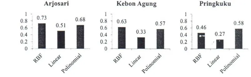
This study was done by making the model at each weather station using three kernels (linear,

polynomial, and RBF). The best model obtained using grid search. Figure 3 show the

comparison of R2 for each kernel and each station.

Arjosari Kebon Agung Pringkuku

I .

~~

;1

0

."

_1°.

68 0';' ---

-<">..«. ~ .~

<'LV_{.•• .~}~V' _{0••••}",,"

-»

-s.,-$'

~O

I -0.8 i 0.63

I

0.6.;zyxwvutsrqponmlkjihgfedcbaZYXWVUTSRQPONMLKJIHGFEDCBA

I

I

0.4 ~ 0.33

0.2

I

° ~--~----~--~~

0.57

I -0.8 I

0.6 ~ 0.46

I

0.4

i

I

0.27

o.~

.J-]

a.:

1

zyxwvutsrqponmlkjihgfedcbaZYXWVUTSRQPONMLKJIHGFEDCBA

_

[image:6.599.70.471.562.686.2]

L.C II~U I U I """1)zyxwvutsrqponmlkjihgfedcbaZYXWVUTSRQPONMLKJIHGFEDCBAJt..~ •.•••• ~ ••••••.••••••••.•••••••_. __ •.••• •••••••

From Figure 3, it can be seen th at the best coefficient detennination at Arjosari weather station obtained when RBF kernel used in the mode ling with the value of R2 is 0.73. The best coefficient detennination at Kebon Agung weather station also obtained when RBF kernel used in the modeling with the value of R2 is 0.63. On the other hand, the best coefficient detcrmination at Pringkuku weather station obtained when polynomial kernel us ed in the modeling with the value of R2 _{is 0.58. The figure also shows that the worst kernel based on its} coefficient

detcrmination

is the linear kernel. It show that model ing using lincar kernel produced results which have the weakest relationship with the actual data.

Arjosari

Kebon

Agung _Pringkuku

5 ₅

4 - 2.86 3.23 3.09

lLLl._J..

Fig.4 Comparison of RMSE for each kernel and each station

(a)

27

41 25zyxwvutsrqponmlkjihgfedcbaZYXWVUTSRQPONMLKJIHGFEDCBA

j 23

~ 21

g

19 ~ 17

"0 15

~13 ~11 9

9 11 13 15 17 1921232527

Actual value

(b)

; 30

---'"

t ~:;~~...

4-· .

.;:&~:

~ 10 ~--.- ---- • --- •••••.•.Prediction

~ 5 _Actual ValuezyxwvutsrqponmlkjihgfedcbaZYXWVUTSRQPONMLKJIHGFEDCBA

~ 0 ~

-OI

...l

02-03 03-04 04-05 05-06 06-07 07-08 08-09 09-10 10-11 11-12 [image:7.597.100.478.202.326.2]

Year

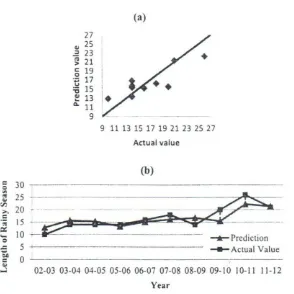
Fig. 5 Comparison between predicted value and actual value in Arjosari station using RBF kernel: (a) scatter piot and (b) line chart

[image:7.597.156.450.366.660.2]

/

zyxwvutsrqponmlkjihgfedcbaZYXWVUTSRQPONMLKJIHGFEDCBA

Figure 4 show the comparison of RMSE for each kernel and each station. Ir show th at the best RMSE at Arjosari, Kebon Agung, and Pringkuku weather station obtained when the model used RBF kernel, with the value of RMSE respectively are 2.45, 3.23, and 2.86. The figure show that the best kernel berween the three kernel is the RBF kernel and the worst kernel is the linear kernel. Ir means that mode ling using RBF kernel gives the least error in predicting the length of rainy scason.

Figure 5 show the comparison berween the length of rainy season value obtained from SVR with RBF kernel and the actual lcngth of rainy season in Arjosari weathers station. It shows that at several periods the predictions are almost accurate while in some periods the prediction

are still overestimated and underestimated.zyxwvutsrqponmlkjihgfedcbaZYXWVUTSRQPONMLKJIHGFEDCBA

Conclusion

The conclusion of this study is the modeling of the length of rainy season based on Southern Oscillation Index and Dipole Mode Index successfully done for each weather station. The best model at Arjosari and Kebon Agung weather station obtained when RBF kernel us ed in the modeling. The best accuracy values obtained are RZ _{of 0.73 and RMSE of 2.45 for Arjosari} weather station, whereas the best accuracy values obtained at Kebon Agung weather station are R1 of 0.62 and RMSE of 3.23. For Pringkuku weather station, the best determination coefficient (R 1) obtained when polynomial kernel used in the modeling with the value of R2 is 0.58. Meanwhile, the best RMSE value at Pringkuku weather station obtained when RBF kernel used in the model ing with the RMSE value is 2.86. The study also concluded that for model ing length of the rainy season, the best kernel to be used is RBF kernel while the worst kernel is the linear kernel.

A cknowledgemzyxwvutsrqponmlkjihgfedcbaZYXWVUTSRQPONMLKJIHGFEDCBAeliI

The authors thank the Directorate of Higher Education, Indonesia for financial support via BOPTN scheme and the Centre for Climate Risk and Opportunity Management in Southeast Asia and Pacific, Bogor Agricultural University (CCROM-SEAP IPB), lndonesia for providing the rainfall data.

References

A. Buono, M. Mukhlis, A. Fakih, R. Boer (2012), Pemodelan jaringan syaraf tiruan untuk prediksi panjang musim hujan berdasar sea surface temperature. Seminar Nasional Aplikasi Teknologi Informasi, Yogyakarta, June, 2012.

A. Buono, LS. Sitanggang, Mushthofa, and A. Kustiyo (2014), Time-delay cascading neural network architecture for mode ling time-dependent predictor in onset prediction, Journal of Computer Science, 10(6), pp. 976-984,2014.

A. Chandrasekar (2010), Basics of Atmospheric Science, PHJ Learning Private Limited, New Delhi, India.

A.J. Smola, B. Scholkopf (2004), A tutorial on Support Vector Regression, Statistics and Computing. 14, pp. 199-222,2004.

C. Chang, C. Lin (2011), UBSVM : a library for support vector machines, ACM Transactions

on lntelligent Systems and Technology, 2(3), 27, 20zyxwvutsrqponmlkjihgfedcbaZYXWVUTSRQPONMLKJIHGFEDCBAII.

S. Behera, P Brandt, G. Reverdin (2013), The tropical ocean circulation and dynamics, Intemational Geophysics Series: Ocean Circulation and Clirnate. 103, pp. 385-404,2013.

R.E. Walpole (1992), Pengantar Statistika (Introduction to Statistics), Gramedia, Jakarta. Indonesia.