Linear Parameter Varying (LPV) Model Identification on Primary Reformer Section of Ammonia Plant for Operator Training Simulator

(1)

Linear Parameter Varying (LPV)

Model Identification on Primary Reformer Section

of Ammonia Plant for Operator Training Simulator

Heri Subagiyo

*

Department of Electronics Engineering Politeknik Caltex Riau, Pekanbaru, Riau, Indonesia

heri@pcr.ac.id

Abstract — System or process identification is the field of mathematical modeling of systems (processes) from test or experimental data. Most of the existing works on process modeling were based on LTI (Linier Time Invariant) model. This paper presents the Linear Parameter Varying (LPV) model identification for primary reforming process in ammonia plant to cover changes in process operating conditions, such as start-up, normal operation and shut-down. Recursive Least Square (RLS) based algorithm with parameter function pk=sin(0.0001*k) is

employed in the identification process. Data needed for identification are taken from DCS historian data of the primary reformer process. The identification result is simulated and validated with the measured data. The process models obtained by this technique show reasonably fit with the mean value of 90.42 %. The process models are implemented on a simulation engine of Operator Training Simulator (OTS) using Scilab/Scicos software tools. Simulation result shows that the indicators of process variable mostly accepted. The mean value of deviations between process variables of simulated models and historian data are 10%, 20%, and 5%, for operation rate 40%, 65%, and 100%.

Key words - Identification, Linear Parameter Varying (LPV) model, Primary Reformer, Operator Training Simulator (OTS).

I. INTRODUCTION

System or process identification is the field of mathematical modelling of systems (processes) from test or experimental data [1]. Process model obtained from identification process can be used for process simulation, analysis and design of control systems, design of safety systems. Most of the existing works on process simulation is based on LTI, which is satisfactory for a number of systems. However, system identification based on LTI model appears to be of limited value when the plant operating conditions significantly varies. One of the effective methods to handle varying operating conditions in the plant is to employ Linear Parameter Varying (LPV) model. LPV constitutes linear dynamic systems whose state space matrices depend on parameters which may vary in time. Such a system was recently studied within the context of gain-scheduling control analysis and design which provides stability and performance guarantee along the trajectory of the varying parameters. More recently, some results of LTI system identification was extended to LPV model.

System identification of primary reforming process in an ammonia plant was recently studied for simulation purpose by the first author in [2], based on LTI model. Simulation result shows that the model obtained was satisfactory for reforming process operation on normal operating condition. Simulation for start-up operating condition has not been successfully conducted as high overshoot step responses appears from several process models which exceeds maximum operation limit, prohibiting the simulation to proceed. A careful observation of reforming process reveals that some nonlinearity occurs in the system.

The term Linear Parameter Varying (LPV) system was originally coined by Shamma dan Athans [3] within the context of gain-scheduling design. LPV model appears in many modeling and control problems, such as aerospace or vehicle system applications [4], stall and surge control of jet engine [5] and flutter suppression [6]. As far the authors concern, application of LPV model identification in reforming process has not been studied.

This paper presents the LPV model identification for reforming process in an ammonia plant based on historical data recorded in a distributed control system (DCS). The LPV model is chosen based on the fact that ammonia plant is operated along several operating conditions (start up, normal, shutdown, and emergency operation) and that in every operating conditions there are parameter changes. LPV identification process is based on Recursive Least Square (RLS), a technique originally developed by Bamieh [7].

The rest of this paper is outlined as follows. In Section 2, Primary Reforming in an ammonia process plant is described. In Section 3, LPV model identification algorithm is presented. In Section 4, results of LPV identification for Primary Reformer are presented. Implementation result of LPV model on simulation engine of Operator Training Simulator (OTS) is described in Section 5. Finally, conclusion is drawn in Section 6.

II. PRIMARY REFORMING PROCESS

(2)

Hydrogen is produced by steam reforming of desulphurized natural process gas in the primary reformer section, whereas N2 is obtained by introducing compressed air into secondary reformer, an autothermal reactor used to further reform the remaining natural process gas.

Fig. 1: Ammonia process

The resulting raw synthesis gas mainly contains H2, N2, carbon monoxide (CO), carbon dioxide (CO2) and steam. CO is converted to CO2 and the additional H2 is produced by water gas shift reaction. In the CO2 Removal section, CO2 is removed from the gas and then sent to Urea Plant. The remaining CO and CO2 are converted into methane (CH4) by reacting them with H2 in the Methanation section. The synthesis gas, mostly contains H2 and N2, is then fed into the Ammonia Synthesis Loop section and converted into ammonia before being sent to Urea Plant.

In the primary reformer section, the natural gas is steam reformed. Heat needed for the reaction is supplied in the form of radiant heat from firing of natural fuel gas. Sensible flue gas heat flow along convection section is used to heat several media in the waste heat recovery [8].

The primary reformer section consists of:

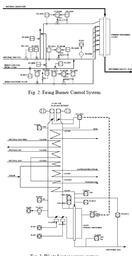
 144 catalyst tube in the two radiant section and side firing burner systems. Firing burner control system is shown in Figure 2.

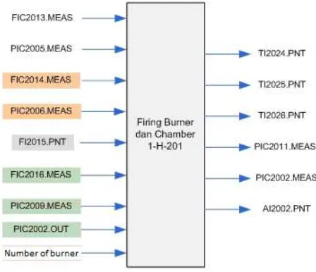
 Waste Heat recovery System (WHS) utilizes sensible flue gas heat produced from primary reformer radiant section in order to heat various coils by convective heat exchange. The system shown in Figure 3 involves:

1. Mixed feed pre-heater coil used to heat hydrocarbon and steam before fed into catalyst tube.

2. Process air heater coil used to heat compressed air before being fed into secondary reformer section. 3. Super heater steam coil used to heat steam to produce

superheated steam.

4. Feed Gas pre-heater coil used to heat natural gas before being fed into desulphurization section. 5. Boiler Feed Water pre-heater coil used to heat boiler

feed water.

Fig. 2: Firing Burner Control System

Fig. 3: Waste heat recovery system

III.LPVMODEL IDENTIFICATION

Linear Parameter Varying (LPV) system is a special class of nonlinear system [9], where the system coefficients are rational function of a parameter. In LPV model, system matrices depends on one or more time-varying parameters and hence represents a family of LTV systems (one for each parameter trajectory) [10].

A discrete time LPV systems represented in the state space form as:

) ( )) ( ( ) ( )) ( ( ) (

) ( )) ( ( ) ( )) ( ( ) 1 (

t u t p D t x t p C t y

t u t p B t x t p A t x

 



(1)

LPV systems model may also be characterized in the form of [7]:

)

(

)

,

(

)

(

)

,

(

p

y

k

B

p

u

k

(3)

where u is input, y is output,



is delay operator, i.e. ) 1 ( : )

(



y _k yk , and

b b n n

p

b

p

b

p

b

p

B

(



,

)



0

(

)



1

(

)









(

)



(3)

a a n n

p

a

p

a

p

A

(



,

)



1



₁

(

)









(

)



(4)

1

  n_a n_b

n is the number of parametric functions to be identified. Assume that the varying parameter p is a function of discrete time (

p



p

(

k

)

).

Parameter function {a_i}, {

b

_i} are assumed to be a linear combinations of a set of known fixed basis functions {f1, ...,

fN}.

)

(

)

(

)

(

p

a

1

f

₁

p

a

f

p

a

N _N

i i

i









(5)

)

(

)

(

)

(

p

b

1

f

₁

p

b

f

p

b

N _N

i i

i









(6)

where the constants k i

a , l i

b are real numbers. Thus any particular model is completely characterized by the real numbers { k

i

a }, and { l i

b }. The goal of a parametric identification scheme in this paper is then to find these constants from process measurement data.

For this general framework, many choices are possible for the function

f

1

(

p

)

. In particular if we consider a polynomial

dependence, then the function are simply powers of p

1 1( )



 l

p p

f

l



1

,...,

N

(7)

In this case the parameter functions are rewritten as

1 2

1

)

(



i



i



iN N

i

p

a

p

a

p

a



(8)

1 2

1

)

(





N N

i i

i

p

b

p

b

p

b



(9)

In recursive least mean square (RLS) identification algorithm it is required to minimize errors between measurement variables and estimation variables which is known as loss function









T k

k

E

T

J

0 2

)

,

(

1

)

(

Θ



Θ

(10)

where

Θ

is n x N matrix that contains coefficients to be identified:















N nb nb N N na na N N

b

a











1 0 1 0 1 2 1 2 1 1 1

:

Θ

(11)

and



(

k

,

Θ

)

, called prediction error, is defined as

k k

y

k

,

Θ

)

Θ

,

Ψ

(







(12)

where yk is measurement data (output of the system) and

k

Ψ

Θ, is estimation output. An extended regressor Ψ, is built by past I/O data and parameter trajectories,



( ) ( ) ( )



:

: 1 2

1 k N k k n k k n k k k k

k f p f p f p

u u y y b a                                

Ψ (13)

In this paper,

Θ

ˆ

_k is parameter coefficients matrix which is estimated at time k. Following RLS algorithm and under appropriate assumption [7], identification algorithm is given by:

)

ˆ

(

trace

,

ˆ

* 1

1 k k k k

k k

k



y



Θ



Ψ



y



Θ



Ψ



(14)

k k k

k

Θ

K



Θ

ˆ



ˆ

_₁



(15)

 

k

P

Ψ

K



(16)

1 1

,

1

_ 

 









_k k k k k k k k

k

Ψ

P

Ψ

P

(17)

where P is covariance matrix expressed in recursive form in Equation (17). Convergence condition of the identification algorithm is attained if Θ₀ is the true value, thus

0

ˆ

lim

Θ



Θ



 k

k (18)

IV.LPVIDENTIFICATION RESULTS

(4)

plant during plant operations. Particular experimentations with some excitation signals are not performed as it will disturb the plant operation process. Data needed for identification process is taken from DCS historian data from February 15, 2006 to March 3, 2006 with sampling time of 1 minutes. All operating conditions of the process (start up, normal, and shut down) are covered in the duration considered. Plots of a sample of historical input signals (TI2010PNT and FIC2001MEAS) are shown in Fig 4. In the subsequent discussions, Prefix T, P and F in various signals identification number represents temperature, pressure and flow, respectively.

Pre-processing of measured data involves data merging, normalization (offset correction) and scaling. Data merging of some measured data is required because, due to limited available storage in DCS, historian data for several operating conditions are not provided in time-successive manner, but instead in time-truncated way. Plots of a sample of data pre-processing results (TI2010PNT and FIC2001MEAS) are shown in Fig 5.

Fig. 4: Sample of measured data: temperature TI2010PNT (upper) and flow FIC2001MEAS (lower)

Fig. 5: Sample of measured data after data pre-processing: temperature TI2010PNT (upper) and flow FIC2001MEAS (lower)

By examining the reformer diagrams and operation described in [8], it is known that Primary Reformer Section process is a multivariable process. All of process can be divided into several sub process, such as Firing Burner System, Primary Reformer, Mixing of Outlet Gas, and Waste Heat recovery System (WHS).

In the following, we present LPV identification results for Firing Burner, Primary Reformer, and Mixing of Outlet Gas - the main subsystems of Primary Reformer.

A.

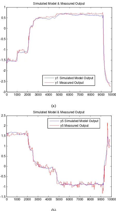
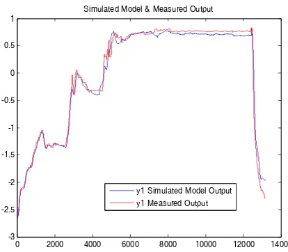
Firing Burner System

Firing Burner System consists of 9 inputs (flows and pressures of natural gas fuel and number of activated burner) and 6 outputs (temperatures and pressures of primary reformer chamber) as shown in Figure 6. For modelling purpose, this MIMO system divided into 6 MISO system, based on number of output, where all input exist in all MISO system. Plot of some simulated LPV model (TI2024PNT and PIC2002 MEAS), along with the corresponding measured data used for identification process is shown in Figure 7.a and Figure 7.b. For TI2024PNT, a best fit of 91.885 and loss function of 0.0066 are obtained. For PIC2002MEAS, a best fit of 88.9707 and loss function of 0.0122 are obtained. Mean best fit for all output is 85.2397. Note that estimated output predict the measured output very well.

Fig. 6: Firing burner input-output

0 1000 2000 3000 4000 5000 6000 7000 8000 9000 -10

-5 0 5

TI2010PNT(Scaled)

0 1000 2000 3000 4000 5000 6000 7000 8000 9000 -3

-2 -1 0 1

FIC2001MEAS(Scaled)

0 1000 2000 3000 4000 5000 6000 7000 8000 9000 100

200 300 400 500

TI2010PNT

0 1000 2000 3000 4000 5000 6000 7000 8000 9000 0

1 2 3x 10

(5)

0 1000 2000 3000 4000 5000 6000 7000 8000 9000 10000 -3

-2.5 -2 -1.5 -1 -0.5 0 0.5 1

Simulated Model & Measured Output

y1 Simulated Model Output y1 Measured Output

(a)

0 1000 2000 3000 4000 5000 6000 7000 8000 9000 10000 -1.5

-1 -0.5 0 0.5 1 1.5 2 2.5

(b)

Fig. 7: Actual/measured and predicted/simulated outputs of Firing Burner System, (a) TI2024PNT output, (b) PIC2002MEAS output

The LPV model obtained is of the form (in MATLAB symbol):

y1(k)=-A1p*y1(k-1)-A2p*y1(k-2)

+B11p*u1(k-1)+B21p*u2(k-1)+B31p*u3(k-1) +B41p*u4(k-1)+B51p*u5(k-1)+B61p*u6(k-1) +B71p*u7(k-1)+B12p*u1(k-2)+B22p*u2(k-2) +B32p*u3(k-2)+B42p*u4(k-2)+B52p*u5(k-2) +B62p*u6(k-2)+B72p*u7(k-2);

where

A1p = Theta1(1,:)*p; A2p = Theta1(2,:)*p; B11p = Theta1(3,:)*p; B21p = Theta1(4,:)*p; B31p = Theta1(5,:)*p; B41p = Theta1(6,:)*p; B51p = Theta1(7,:)*p; B61p = Theta1(8,:)*p; B71p = Theta1(9,:)*p; B12p = Theta1(10,:)*p; B22p = Theta1(11,:)*p; B32p = Theta1(12,:)*p; B42p = Theta1(13,:)*p; B52p = Theta1(14,:)*p; B62p = Theta1(15,:)*p; B72p = Theta1(16,:)*p;

y1 = TI2024PNT;

u1…u7 = all input of firing burner

and

p=[1; sin(0.0001*k); (sin(0.0001*k))^2];

Theta1 is 16x3 matrix representing identified parameters as shown below.

Theta1 =[

-0.7274 -0.0991 -0.0540 -0.2397 0.0770 0.0510 0.0051 0.0019 0.0021 -0.0015 -0.0026 -0.0004 -0.0016 -0.0041 0.0009 0.0284 0.0116 0.0069 0.0013 -0.0013 -0.0002 0.0056 0.0028 -0.0003 0.0191 -0.0042 -0.0013 -0.0053 -0.0056 -0.0036 0.0042 0.0006 0.0026 -0.0146 -0.0059 -0.0015 -0.0115 -0.0130 -0.0070 0.0004 -0.0014 -0.0001 -0.0088 -0.0001 -0.0007 0.0127 -0.0016 0.0007]

The LPV model obtained is of the following form:

y5(k)=-A1p*y5(k-1)-A2p*y5(k-2)

+B11p*u1(k-1)+B21p*u2(k-1)+B31p*u3(k-1) +B41p*u4(k-1)+B51p*u5(k-1)+B61p*u6(k-1) +B71p*u7(k-1)+B12p*u1(k-2)+B22p*u2(k-2) +B32p*u3(k-2)+B42p*u4(k-2)+B52p*u5(k-2) +B62p*u6(k-2)+B72p*u7(k-2);

where

A1p = Theta5(1,:)*p; A2p = Theta5(2,:)*p; B11p = Theta5(3,:)*p; B21p = Theta5(4,:)*p; B31p = Theta5(5,:)*p; B41p = Theta5(6,:)*p; B51p = Theta5(7,:)*p; B61p = Theta5(8,:)*p; B71p = Theta5(9,:)*p; B12p = Theta5(10,:)*p; B22p = Theta5(11,:)*p; B32p = Theta5(12,:)*p; B42p = Theta5(13,:)*p; B52p = Theta5(14,:)*p; B62p = Theta5(15,:)*p; B72p = Theta5(16,:)*p; y5= PIC2002MEAS;

u1…u7 = all input of firing burner

and

p=[1; sin(0.0001*k); (sin(0.0001*k))^2];

Theta5 is 16x3 matrix representing identified parameters as shown below.

Theta5 =[

(6)

-0.0422 -0.0180 -0.0151 -0.0179 0.0046 0.0086 -0.0083 -0.0047 -0.0072 -0.1261 -0.0295 -0.0205 0.0114 0.0125 0.0088 0.0039 0.0076 0.0041 -0.0067 -0.0051 -0.0050 0.0312 0.0193 0.0138 0.0108 -0.0054 -0.0094 0.0039 0.0107 0.0080 0.1211 0.0324 0.0209 -0.0115 -0.0113 -0.0103]

B.

Primary Reformer (1-H-201)

Primary Reformer consists of 11 inputs (flow, temperature, and pressure of steamed natural gas, and temperature of primary reformer chamber) and 9 outputs (temperature and pressure of the result of primary reforming process) as shown in Figure 8. Similar to Firing Burner system, this MIMO system divided into 9 MISO systems. Plot of a simulated LPV model (TI2027APNT), along with the corresponding measured data used for identification process is shown in Figure 9. A best fit of 90.6615 and loss function of 0.0087 are obtained. Mean best fit for all output of Primary Reformer (1-H-201) is 94.2617. Note that estimated output predict the measured output very well.

Fig. 8: Primary Reformer (1-H-201) input-output

0 2000 4000 6000 8000 10000 12000 14000 -3

-2.5 -2 -1.5 -1 -0.5 0 0.5 1

Fig. 9: Actual/measured and predicted/simulated output of Primary Reformer (TI2027APNT output)

The LPV model obtained takes the following form:

y1(k)=-A1p*y1(k-1)-A2p*y1(k-2)

+B11p*u1(k-1)+B21p*u2(k-1)+B31p*u3(k-1) +B41p*u4(k-1)+B51p*u5(k-1)+B61p*u6(k-1) +B71p*u7(k-1)+B81p*u8(k-1)+B91p*u9(k-1) +B101p*u10(k-1)+B111p*u11(k-1)+B12p*u1(k-2) +B22p*u2(k-2)+B32p*u3(k-2)+B42p*u4(k-2) +B52p*u5(k-2)+B62p*u6(k-2)+B72p*u7(k-2) +B82p*u8(k-2)+B92p*u9(k-2)+B102p*u10(k-2) +B112p*u11(k-2);

C.

Gas Mixing (1-H-201 Outlet)

Mixing of Outlet Gas consists of 4 inputs (temperature of results of primary reforming process) and 1 output (mixed temperature of the result of primary reforming process) as shown in Figure 10. Plot of simulated LPV model, along with the corresponding measured data used for identification process is shown in Figure 11. A best fit of 90.6615 and loss function of 0.0087 are obtained. Note that estimated output predict the measured output very well.

The model development procedure in this example can be used for the other sub-process of primary reformer section. The mean values of best fit for all sub-process is 90.42 % which are moderately accepted.

(7)

0 2000 4000 6000 8000 10000 12000 14000 -3

-2.5 -2 -1.5 -1 -0.5 0 0.5 1

Simulated Model Output Measured Output

Fig. 11: Actual/measured and predicted/simulated output of Gas Mixing (TI2028PNT output)

The LPV model obtained takes the following form: y1(k)=-A1p*y1(k-1)-A2p*y1(k-2)+B11p*u1(k-1)

+B21p*u2(k-1)+B31p*u3(k-1)+B41p*u4(k-1) +B12p*u1(k-2)+B22p*u2(k-2)+B32p*u3(k-2) +B42p*u4(k-2);

Several remarks on varying parameter are in order. The varying parameter used in the identification process described above is sinusoidal function of sufficiently small frequency to obtain satisfying results. Although not shown, we noticed in our experiments that the use of higher frequencies tends to produce smaller best fit. It seems to the authors that such a result is due to the fact that the ammonia process is sufficiently slow.

V. MODEL IMPLEMENTATION

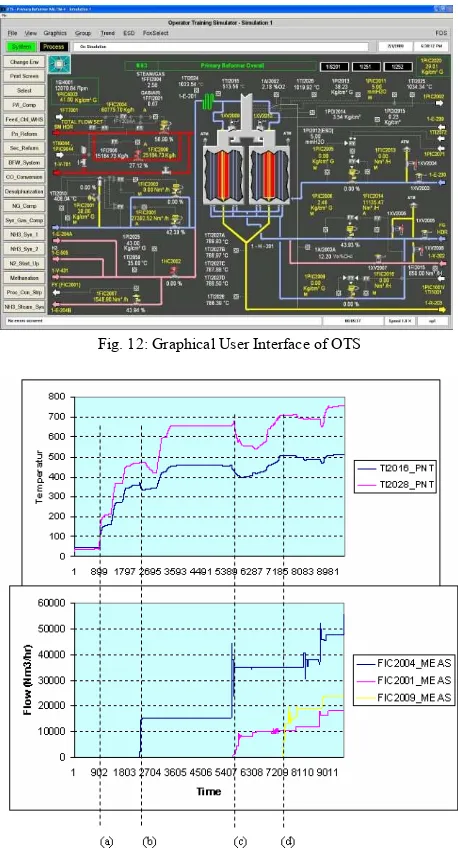
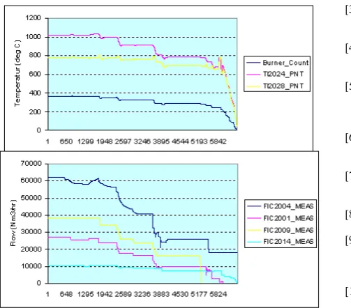
The process models are implemented on a simulation engine of Operator Training Simulator (OTS) using Scilab/Scicos software tools. Graphical User Interface (GUI) of OTS is developed using Wonderware InTouch®. A display of GUI is shown in Figure 12. The OTS dynamically simulated for start-up, normal, and normal shutdown training scenarios. Plot of some important process variable indicator (TI2016PNT, TI2028PNT, FIC2004MEAS, FIC2001MEAS and FIC2009MEAS) during these scenarios shown on Figure 13, and Figure 14.

Fig. 12: Graphical User Interface of OTS

Fig. 13: Plot of some process variable indicator during start-up scenario, (a) Firing Burner activated, (b) steam/FIC2004MEAS is fed, (c) natural gas is fed,

and (d) process air is fed.

(8)

Figure 14: Plot of simulation result for normal shutdown scenario

VI.CONCLUSION

This paper presents the LPV model identification for primary reformer section of ammonia plant. In general, the models obtained by using the LPV model identification with Recursive Least Square (RLS) algorithm and parameter trajectory sequence

p

_k



sin(

0

.

0001

*

k

)

, show reasonably fit with the mean value of 90.42 %. This is satisfactory result for further work on the LPV control system application or Process Simulator. After implementation of process model on simulation engine of Operator Training Simulator (OTS), the mean value of deviations between process variables of simulated models and historian data are 10%, 20%, and 5%, for operation rate 40%, 65%, and 100%.

The model development and implementation procedure in this paper can be used for the other sections of ammonia plant. For future works, the parameter function determination of LPV model has to be researched to produces more systematically determination.

ACKNOWLEDGEMENTS

The authors are grateful to staff of PT. Pupuk Kaltim, Tbk who provide DCS historian data needed

REFERENCES

[1] Zhu, Yucai, Multivariable System Identification for Process Control, Oxford: Pergamon, 2001.

[2] Erwin Hendarwin, Development of Operator Training Simulator for Ammonia Plant (Process Modeling, Control and Simulation), Master Thesis, Electrical Engineering Department, Institut Teknologi Bandung, Januari 2006.

[3] J. Shamma and M. Athans, “Guaranteed properties of gain scheduled control for linear parameter varying plants”, Automatica, Vol. 27 No. 3, 1991, pp. 559-564.

[4] J. Bokor and G. Balas, "Linear parameter varying systems: A geometric theory and applications", Preprints 16th IFAC World Congress, Prague, Czech Republic, July 2005, pp. 69-79.

[5] B. Bamieh, L. Giarr´e, T. Raimondi, D. Bauso, M. Lodato and D. Rosa,

“LPV Model Identification For The Stall And Surge Control Of Jet Engine”, 15th IFAC Symposium on Automatic Control in Aerospace,

Bologna, Italy, September 2001.

[6] H.Y Sutarto* and M.Fadly, “LPV Model Identification for Flutter

Suppression Application”, Proc. of the 6th Asian Control Conference

(ASCC), Bali, Indonesia, 2006.

[7] B. Bamieh, L. Giarre, “Identification of Linear Parameter Varying

Models”, International. Journal of Robust and Non-Linear Control, Vol. 12, 2002, pp. 841-853.

[8] Nugraha B.E. Irianto, Kaltim-4 Ammonia Plant Operation Guide, PT. Pupuk Kalimantan Timur, Tbk, Bontang, 2002.

[9] M. Nemani, R. Ravikanth, B.A. Bamieh, ”Identification of Linear

Parametrically Varying Systems”, Proc. of the 34th IEEE Control and Decision Conference Vol. 3, New Orleans, Lousiana, December 1995, pp. 2990-2995.

[10] L.H. Lee, K. Polla, “Identification of Linear Parameter-Varying

Systems via LFTs”, Proc. of the 35th Conference on Decision and

Control, Kobe, Japan, December 1996.