Application of Uncorrelated Leaning from Low-rank Dictionary in Blind Source Separation

DOI: _{10.12928/TELKOMNIKA.v14i2A.4319}  ₂₅₇

Application of Uncorrelated Leaning from Low-Rank

Dictionary in Blind Source Separation

Liu Sheng*1, Zhou Shuanghong2, Li Bing3, Zhang Lanyong4 1,3,4

College of Automation, Haerbin Engineering University, Haerbin Heilongjiang, 150001China 2_{College of Science, Haerbin Engineering University, Haerbin Heilongjiang, 150001 China}

*Corresponding author, e-mail: 37645694@qq.com

Abstract

This paper proposes a kind of method about signal BOA estimation from the aspect of sparse decomposition. The whole interested space is divided into several potential angles of arrival to establish a over-complete directory to convert the estimation problem of signal DOA to sparse representation problem. A MMV array is formed by data received from multiple snapshots, then using optimization method of joint sparse constraint to solve the problem. First, make singular value decomposition on received data array to connect the each snapshot data, then using the sparse representation problem of bounded to solve the problem. To improve the anti-noise performance of algorithm, the paper applies similar Sigmoid function of two parameters to approximate norm. This method applies to the DOA estimation of narrow-band and broad-band signal. shall be used for solving MMV problem, which achieves joint sparse constraint of all frequency of reception matrix of broadband signal, to make array elements spacing break through the limitation of half wavelength and improve resolution of DOA signal.

Keywords: Blind source; Source separation; Joint sparse; Smooth norm

1. Introduction

2. Model Construction 2.1. Signal Model

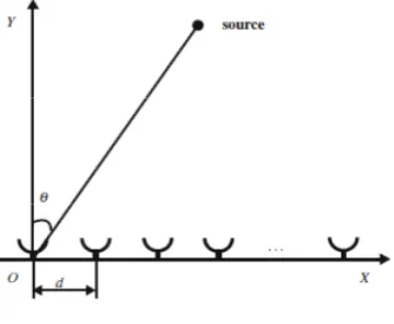
The object of estimation of signal DOA is to find the angle of arrival incident on signal source of array. Known information includes geometric construction of array, parameter of medium of signal transmission, received data of array element. This section firstly considers the DOA estimation of narrow-band signal and DOA estimation of broadband signal will be discussed in next section.

Figure 1. ULA receiving array

Considering ULA array shown in Figure 1. M of each isotropic receiving array receives

K of remote field static incident signal. The most left array element is reference array element, distance of array element is _/ ,  is the wave length. The angle of incident of is

Received signal of array element can be expressed as the following linear equation:

 

   

 

y t  A  s t w t (1)

In which, y t

 

 _y t y₁

   

₂ t ...y_M

 

t _T is received signal vector, w t

 

unknown noise

vector and s t

 

 s t s₁

   

₂ t ...sK

 

t Tis vector of signal source. A

 

  a

     

1 a 2 ...a K  is

oriented matrix, in which, a

 

k is vector of length M and

 

  1 sin

, 1, 2,...

k

j m km

a  e   m M.

Estimation problem of signal DOA is the direction of angle  

 

k of signal source that

estimated by received signal vector y t

 

.

In spite of DOA estimation based on single snapshot data has its application values, DOA estimation with multi-snapshot data may occur in actual application frequently. Considering the time sampling is formula (1), narrow-band signal DOA estimation problem with multi-snapshot data may be expressed as:

 

 

Y A θ S W ₍₂₎

In which, Y Y

   

t1 Y t2 ...Y

 

tJ , J is snapshot number. The definition of S and W

is the same as Y_.

2.2. DOA Estimation Expressed on the Basis of Sparse Directory

To transform DOA estimation into a sparse representation problem, all possible over-complete angle of arrival shall be introduced to express A_{. Firstly, dividing the whole interested}

all potential angle of arrival can be used for constructing a over-complete oriented matrix

     

1 2 .... N

a  a  a 

 

  

Φ . Φis known and not relevant to DOA of actual signal source.

1

N vector quantity S

 

tj shall be expressed as location of signal sources; and when

n k

  , n element of S

 

tj is non 0, or it is 0. DOA information signal source can be obtained

from the location of non 0 value of S

 

tj . Of course, DOA of actual signal may not be equal to

certain _n all the time. However, if is enough intensive, thus certain _n exists to make_n_k; existing deviation can be expressed approximately as noise. Analyzing from the above, the DOA estimation of signal can be expressed as: Y =ΦS + W

For only considering the situation of static signal in this paper, DOA of signal is a time-invariant vector in the whole measuring progress; each line of non 0value in matrix S_is

appeared in the same line. In other words, only Kbehavior is non 0in matrix S_{. Therefore,}

DOA estimation of signal can be expressed as MMV problem of joint sparse matrixS_{is found by}

observation dataY.

3. DOA Estimation of Narrow-Band Signal

3.1. Multiple Parameter Approximation

The standard to evaluate performance of approximate function of norm mainly includes two aspects: noise tolerance and the accuracy of approximation. It is assumed that is the approximate function of norm, there are two parameters can be used for expressing the property of . g w

 

|w0.5 is used for describing the noise tolerance of

approximate function and is used for describing the accuracy of function of approximation; in which, g w

 

 f1

 

x . When system dimension is higher, w_c 



m1 /



m (in which, is the dimension of signal source) can be selected as the dimension of signal sources. Expectation  can be adjusted according to noise and the adjustment of  not affected by  in noise environment.

Up to now, Gaussian function

 

2 2

2 x

f x e  is used generally as the approximate

function [13] of l0norm. For Gaussian function, there is

(3)

(4)

Obviously, both of  and depend on . The adjustment of  can affect on  inevitably, so that noise tolerance performance of approximate function is reduced.

The disadvantage of one-parameter approximate function can be avoided by selecting approximate function of multi parameters. The paper selects a kind of approximate function of two-parameter that is similar to Sigmoid function:

 

2

2

,

2 1

1

u _{x u}

f x

e





  



(1)

For f,u

 

x , there is

 





0.5 1

|_w u, |_{w m m} 2 ln m 1 u

 _   _{ }    (2)









2 2 ln 2

2 ln m 1 m

 

 



Obviously, only can be determined by parameter , and adjustment of can be achieved through . In other words, the noise tolerance of _, and accuracy of approximation can be determined by different parameters.

3.2. Blind Source Separation for Measurement Matrix

In practical application, the dimension of measurement matrix is so high that reaches hundreds or thousands. In order to reduce the complexity of calculation and the sensibility to noise, the singular value decomposition for measurement Y is initially needed. The singular value decomposition is designed to decompose the measurement matrix into subspaces of signal and noise, and only retain the subspace of signal, thus transforming the estimation issue of signal DOA into MMV issue which has lower dimension.

By only retaining the subspace of signal, the measured data



 



1 J j j t 

Y _{shall turn into a}

K dimension signal, where K is the number of signal source. The singular value decomposition of measurement matrix Y can be expressed as

'

Y = ULV ₍₇₎

Where Ysvis MKdimension matrix which including substantially all energy of signal.

TheYsv can be expressed as Ysv ULDK YVDK, in which DK 



IK 0



. Meanwhile, both Ssv

and Wsv can be expressed as Ssv SVDk andWsv WVDK, and then sv  sv sv

Y ΦS W

The formula (8) and formula (2) have the same expression, except the dimension drops from J to K, which enables the estimation method of signal DOA which is based on sparse representation to have better instantaneity.

3.3. Estimation Method of DOA Constrained by Smooth

By using the approximate function of norm defined by formula (5), the sparseness of signal source vector can be expressed as

 



 



, , ₂

1

,:

N

u u

i

F N f i



 



S S ₍₈₎

Therefore, if the measured data Y is known, the signal source vector S can be solved by following formula:

(9)

(10)

Whereuis the constant relevant to noise, and  is the number approximate to 0, and

 

2 2

2 F

A  vec A is the Frobenious norm of matrix A. The parametercontrols the sparseness of

signal and the compromise of noise level.

Asu_{is in correlation with noise level, it can be considered as a constant here. When} _is low, the sparseness of signal source vector S approximate to functionF,u

 

S and has many

local minimum points; with the growth of, f,u

 

S shall become smoother and smoother.

When  , there is





_*



_*



1

* lim , u S u   

 Φ ΦΦ Y (3)

Where * is the conjugate transposition of matrix . So the formula (10) can be solved by regarding a bigger  value as initial point; then reduce the  value constantly, and then solve







 



 

 

,

2

, ,

, arg min _u ,

s

u u F

u L L F          S S

formula (10) until condition of convergence is reached. In order to solve formula (10), the paper adopted an algorithm similar to Gaussian-Newton.

In which, as for fixed , , the definition for is as follows:

(12)

(13)

Then there is S*



,u







S*



,u





. Beyond that, for any signal source vector S, there

existing actual value scalar  0, which shall meet

  







 

,u 1 ,u

L_  S   S L_ S ₍₄₎

Because of S*



,u







S*



,u





, the answerS*



,u



of signal source vector can be

got from formulaS*



,u







S*



,u





by adopting method of iteration for fixed points. To ensure

the convergence of algorithm L,u





 

S



L,u

 

S must be met. However, not all S shall meet

this, so it can be solved through formula (14). The whole flow of algorithm is as follows: Initialize:

(1) Assume_S 0 _{Φ ΦΦ}*



*



1_Y;

(2) Estimate the noise level by method in document, and then determine the parameter

uaccording to noise level. Assume  0

 

2

max ,:

i i

  S _;_1,   _{, ,} 

 

_{0,1 ,}

0 1e 4

   .

(3) Measure the singular value deposition of matrix Y. When  0, repeat:

(4) Let 1;

;

 

(5) Complete until L,u





  

S  1 



S



L,u

 

S   ;

(6) S i1 

 

S i  



1 



S i

(7) If then

4. Results and Discussion

This section shall verify the effectiveness of method adopted by this paper by comparing all kinds of different DOA estimation method such as algorithm ofMixed l2,0,l1SVD,

MUSIC and CAPON. The estimation of parameterushall adopt method proposed in document. The ULA array of array element number M=16 shall be adopted and the space between array elements is half wavelength of narrow-band signal. Uncorrelated signal is to be considered primarily. The amplitude of narrow-band signal shall meet Gaussian distribution of

mean value

0

. Disperse the whole space domain_0 ,180 _into grid point with resolution of 1, i.e. N = 181, _ΦCM N _{. Measure the effect of uncorrelated noise which the signal subjects in}

time domain and space domain. Firstly select the fixed number of snapshots, like J = 100. The effect which the number of snapshots made on rebuilding results shall be discussed below.

 

 

 

 

 





 

 





2 2 ,: 2 2 2 1 0 0 1 1

0 ... 0

0 0

1 S i u

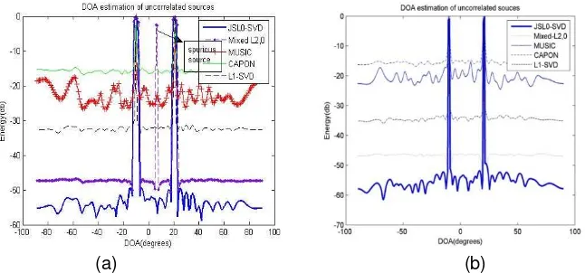
Figure 2 describes the spatial spectrum got by each of different algorithms when the space between grid points is 1 and 0.5. The signal to noise ratio SNR10db and the directions of signal source are -10 and 20.7, and they are not correlated. Figure 2(a) describes the result when the space of grid point is1. Although the DOA of the second signal source has

not exactly fallen over the grid point, it can be observed that a signal source can be got at 21 from the closest real value of signal source DOA byJSL0SVDalgorithm. Figure 2(b) describes

the result when the space between grid points is0.5. It can be observed from the figure that

reducing the space between grid points cannot evidently improve rebuilding quality. Figure 2(a) and (b) indicate that all methods can be used to recognize two targets, but sometimesl1SVD

andMixed l2,0shall receive spurious signal source, especially when SNR is low.

[image:6.595.137.460.245.396.2]

(a) (b)

Figure 2. Estimation of uncorrelated signal DOA: (a) gird °, (b) gird .5°

Figure 3 describes the DOA estimation result when correlation coefficient is 0.95 and arrival angles are 60and80respectively.

From the figure, it can be observed that all methods on the basis of sparseness representation is able to accurately estimate the arrival angle of signal source, butl1SVDand

2,0

Mixed l also may get spurious target signal source. If the signal sources number is unknown

or SNR is low, l1SVDshall get spurious signal source; if SNR is low, Mixed l2,0shall get

spurious signal source. If the number of snapshots is small, the algorithms of MUSIC and CAPON are unable to effectively estimate the DOA of target signal.

[image:6.595.142.452.575.727.2]

(a) (b)

Next we analyze the effect of the number of snapshots on the performance of different DOA estimation algorithms. In the simulation, two strong correlated signals from different directions shall be used with SNR10db, and by changing number of snapshots, the effect of the number of snapshots on algorithm performance can be verified. 500 times of independent simulation shall be done for each snapshot value. If MSE of the simulation result is lower than some fixed threshold, then it shall be deemed as failing to accurately estimate the DOA of signal. Figure 4(a) is the simulation result. Due to the number of snapshots required by estimation method basing on sparse representation is far lower than the number of snapshots required by algorithms of MUSIC and CAPON, the performance curve of algorithms of MUSIC and CAPON has not been drawn in the simulation. The figure shows that the performance of

0

JSl SVD is evidently superior to Mixed l2,0 and l1SVD. Figure 4(b) described the effects of

SNR have on estimation performance by each algorithm. In this simulation, the SNR value shall be changed while other values shall retain. Because l1SVD and Mixed l2,0 shall generate

spurious signals when SNR is low, so the performance of is obviously superior to the other two methods. When SNR is high, the performance of and is quite approximate.

[image:7.595.124.468.293.458.2]

(a) (b)

Figure 4. Influence of Number of Snapshots and SNR on DOA Estimation Performance: (a) Number of snapshots on DOA estimation performance

(b) SNR on estimation performance

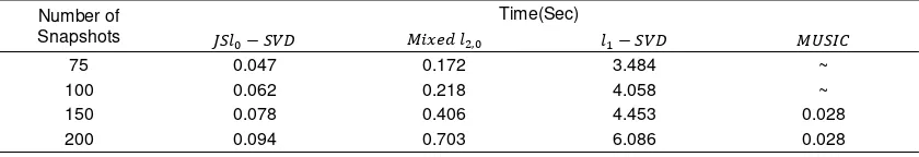
Finally, we shall compare the computational efficiency by each of different algorithms. For the algorithm of MUSIC is unable to effectively estimate DOA of correlated signal, the simulation shall use uncorrelated signals with fixed SNR and changeable numbers of snapshot, and the result is showed in Figure 1. Although the computational efficiency of algorithm of MUSIC is the highest, it also should be noted that DOA estimation performance by algorithm of MUSIC is for lower than that by method based on sparseness representation. The computational efficiency of l1SVD and Mixed l2,0 is lower than JSl0SVD. This is because

the efficiency of two-level cone planned algorithm of sparseness representation issue constrained by resolution l1is low, and also because is seeking for sparseness solution in the

whole space and the computational efficiency is low when the dimension of signal is high.

Table 1. Comparison of computational efficiency

Number of Snapshots

Time(Sec)

,

75 0.047 0.172 3.484 ~

100 0.062 0.218 4.058 ~

[image:7.595.88.508.685.757.2]

5. Conclusion

This paper transforms the estimation issue of signal DOA into a solution issue combined with sparseness representation. By the singular value decomposition of received data matrix, the combination of numbers of snapshots of each time and frequency has been achieved; then the estimation of signal source DOA has been realized by solving a combined optimization issue constrained by smooth norm sparseness. The signal DOA estimation method based on sparseness representation not only can reduce data size effectively, but also has following merits: better anti-noise performance; higher computational efficiency; applicable to correlated and uncorrelated signals. By comparing with other DOA estimation methods, the effectiveness and superiority of methods in this paper has been proved. In addition to this, also has some merits as follows: better anti-noise performance; higher computational efficiency; applicable to correlated and uncorrelated signals.

References

[1] Jinyu Hu and Zhiwei Gao. Distinction Immune Genes of Hepatitis-induced Heptatocellular Carcinoma. Bioinformatics. 2012; 28(24): 3191-3194.

[2] Song X, Geng Y. Distributed Community Detection Optimization Algorithm for Complex Networks.

Journal of Networks. 2014; 9(10): 2758-2765.

[3] Pahlavan K, Krishnamurthy P, Geng Y. Localization Challenges for the Emergence of the Smart World. Access. IEEE.2015; 3(1): 1-11.

[4] Song X, Geng Y. Distributed Community Detection Optimization Algorithm for Complex Networks.

Journal of Networks. 2014; 9(10): 2758-2765.

[5] Pahlavan K, Krishnamurthy P, Geng Y. Localization Challenges for the Emergence of the Smart World. Access. IEEE. 2015; 3(1): 1-11.

[6] He J, Geng Y, Wan Y, Li S, Pahlavan K. A Cyber Physical Test-bed for Virtualization of RF Access Environment for Body Sensor Network. Sensors Journal. IEEE. 2013; 13(10): 3826-3836.

[7] Jiang D, Xu Z, Lv Z. A Multicast Delivery Approach with Minimum Energy Consumption for Wireless Multi-hop Networks. Telecommunication Systems. 2015: 1-12.

[8] Lin Y, Yang J, Lv Z, Wei W, Song H. A self-assessment Stereo Capture Model Applicable to the Internet of Things. Sensors. 2015; 15(8): 20925-20944.

[9] Ying Liang. Satisfaction With Economic and Social Rights and Quality of Life in a Post-Disaster Zone in China: Evidence From Earthquake-Prone Sichuan. Disaster Medicine and Public Health Preparedness.2015; 9(2):111-118.

[10] T Sutikno, D Stiawan, IMI Subroto. Fortifying Big Data infrastructures to Face Security and Privacy Issues. TELKOMNIKA (Telecommunication Computing Electronics and Control). 2014; 12(4): 751-752.

[11] Ying Liang. Correlations between Health-Related Quality of Life and Interpersonal Trust: Comparisons between Two Generations of Chinese Rural-to-Urban Migrants. Social Indicators Research. 2015; 123(3): 677-700.

[12] Ying Liang, Demi Zhu. Subjective Well-Being of Chinese Landless Peasants in Relatively Developed Regions: Measurement Using PANAS and SWLS. Social Indicators Research. 2015; 123(3): 817-835.