A 4-Point Block Method For Solving Higher Order Ordinary Differential Equations Directly.

(1)

Research Article

A 4-Point Block Method for Solving Higher Order

Ordinary Differential Equations Directly

Nazreen Waeleh

1

and Zanariah Abdul Majid

2,3

1_{Faculty of Electronic & Computer Engineering, Universiti Teknikal Malaysia Melaka (UTeM), 76100 Melaka, Malaysia}

2_{Department of Mathematics, Faculty of Science, Universiti Putra Malaysia, 43400 Serdang, Selangor, Malaysia}

3_{Institute for Mathematical Research, Universiti Putra Malaysia, 43400 Serdang, Selangor, Malaysia}

Correspondence should be addressed to Nazreen Waeleh; nazreen@utem.edu.my

Received 18 April 2016; Revised 23 June 2016; Accepted 30 June 2016

Academic Editor: Harvinder S. Sidhu

Copyright © 2016 N. Waeleh and Z. Abdul Majid. his is an open access article distributed under the Creative Commons Attribution License, which permits unrestricted use, distribution, and reproduction in any medium, provided the original work is properly cited.

An alternative block method for solving ith-order initial value problems (IVPs) is proposed with an adaptive strategy of implementing variable step size. he derived method is designed to compute four solutions simultaneously without reducing the problem to a system of irst-order IVPs. To validate the proposed method, the consistency and zero stability are also discussed. he improved performance of the developed method is demonstrated by comparing it with the existing methods and the results showed that the 4-point block method is suitable for solving ith-order IVPs.

1. Introduction

Many natural processes or real-world problems can be trans-lated into the language of mathematics [1–4]. he mathe-matical formulation of physical phenomena in science and engineering oten leads to a diferential equation, which can be categorized as an ordinary diferential equation (ODE) and a partial diferential equation (PDE). his formulation will explain the behavior of the phenomenon in detail. he search for solutions of real-world problems requires solving ODEs and thus has been an important aspect of mathematical study. For many interesting applications, an exact solution may be unattainable, or it may not give the answer in a convenient form. he reliability of numerical approximation techniques in solving such problems has been proven by many researchers as the role of numerical methods in engineering problems solving has increased dramatically in recent years. hus a numerical approach has been chosen as an alternative tool for approximating the solutions consistent with the advancement in technology.

Commonly, the formulation of real-world problems will take the form of a higher order diferential equation asso-ciated with its initial or boundary conditions [4]. In the literature, a mathematical model in the form of a ith-order diferential equation, known as Korteweg-de Vries (KdV) equation, has been used to describe several wave phenomena depending on the values of its parameters [2, 3, 5, 6]. he KdV equation is a PDE and researchers have tackled the problem analytically and numerically. It is also noted that in certain cases by using diferent approaches the KdV might be transformed into a higher order ODE [7]. To date, there are a number of studies that have proposed solving ith-order ODE directly [8, 9]. Hence, the purpose of the present paper is to solve directly the ith-order IVPs with the implementation of a variable step size strategy. he ith-order IVP with its initial conditions is deined as

�v

= � (�, �, ��, ��, ��, �iv

) , � (�) = �0, ��(�) = �1, ��(�) = �2, ��(�) = �3, �iv(�) = �4, � ∈ [�, �] . (1)

(2)

Conventionally, (1) will be converted to a system of irst-order ODEs by a simple change of variables. However, it will increase the computational cost in terms of function evaluation and thus will afect the computational time. his drawback is obviously seen when dealing with a higher order problem. Furthermore, [10] also has remarked that the block method is far more cost-efective when it is implemented in direct integration. Hence, several researchers [11–16] have shown an interest in the development of direct integration methods. A direct integration method of variable order and step size for solving systems of nonstif higher order ODEs has been discussed in [11] whereby [12] has proposed an algorithm based on collocation of the diferential system at selected grid points for direct solution of general second-order ODEs. In addition, [13] has used the Gaussian method in order to solve fourth-order diferential equations directly. However, it requires a tedious computation as well, since it consists of higher order partial derivatives of Taylor series algorithm which supplies the starting values. Jator and Li [15] have proposed the linear multistep method (LMM) for solving general second-order IVPs directly. he method is self-starting, so it involves less computational time by avoiding incorporating subroutines to supply the starting values.

hus far, a number of researchers have concerned them-selves with developing a numerical method based on block features, and the characteristic feature of the block method is that in each application it generates a set of solutions concurrently [10]. Rosser [10] also has remarked that the implementation of block method in numerical computa-tion will reduce the computacomputa-tional cost by reducing the number of function evaluations. Shampine and Watts [17] have constructed an�-stable implicit one-step block method and Cash [18] has studied block methods based upon the Runge-Kutta method for the numerical solution of nonstif IVPs. Furthermore [19] has used the self-starting LMM to solve second-order ODEs in a block-by-block fashion and recently [20] has constructed a predictor-corrector scheme 3-point block method with the implementation of variable step size. his research is an extension of the work in [20] in which the solution is computed at three points concurrently and it shows the satisfactory numer-ical results obtained when solving general higher order ODEs.

An increasing amount of literature is devoted to vari-able step size implementations of numerical methods [11, 21, 22]. he practicality of varying the step size for block method has been justiied by [10]. his strategy is an attempt to reduce the computational cost as well as maintaining the accuracy. he Falkner method with variable step size implementation for the numerical solution of second-order IVPs has been employed in [21]. Although the implemen-tation of the method involves varying the step size and solving directly, the computation is still tedious since the coeicients of the formulae must be calculated every time the step size is changed. On the contrary, the present work will store all the integration coeicients in the code in order to avoid the tedious calculations of the divided diferences.

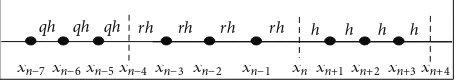
qh qh qh rh rh rh rh h h h h

xn−7 xn−6xn−5xn−4 xn−3 xn−2 xn−1 xn xn+1 xn+2 xn+3xn+4

Figure 1: 4-point block method.

2. Methodology

2.1. Derivation of 4-Point Block Method. he basic approach

of numerical methods for integration is performed by sub-dividing the interval of integration into certain subintervals. he proposed method was based on concurrent computation; hence the closed inite interval was subdivided into a series of blocks and each block contains four equal subintervals as illustrated in Figure 1.

Initially, (1) was integrated ive times over the corre-sponding interval:[�_�, �_�+1],[�_�, �_�+2],[�_�, �_�+3],[�_�, �_�+4] for irst, second, third, and fourth point, respectively. he integration was started by replacing the function

�(�, �, ��, ��, ��, �iv

)with the interpolating function which was generated from Lagrange polynomials. A set of points

{(��−7, ��−7), . . . , (��, ��)}, {(��−4, ��−4), . . . , (��+4, ��+4)} was

interpolated for deriving predictor and corrector formulae, respectively. Let the Lagrange polynomial,�_�(�), be written as

��(�) = ��,0(�) � (��+4) + ��,1� (��+3) + ⋅ ⋅ ⋅

+ ��,�� (��+4−�) = �

∑

�=0��,�(�) � (��+4−�) ,

(2)

where

��,�(�) = �

∏

�=0 � ̸=�

(� − ��+4−�)

(��+4−�− ��+4−�)

for each � = 0, 1, . . . , �. (3)

Nine points were interpolated in (2) with � set to be eight for deriving the corrector and thus one point less for the predictor formula. hen, the integration process was proceeded by substituting� = (� − �_�+4)/ℎand�� = ℎ�� in (2). Consistent with the number of interpolation points involved in deriving the formulae, predictor and corrector formulae were obtained in terms of variables� and �. he variables�and�refer to the distance ratio between current and previous point as a result of implementation variable step size strategy in the proposed method.

In this work, the selection of the next step size could be increased by a factor of(� = 0.5, � = 0.5) or maintained by((� = 1, � = 1), (� = 1, � = 2), (� = 1, � = 0.5))and

(3)

the computation [10]. he compact form of the 4-point block method is presented in

�(v−�)

where�_�,�� are the coeicients of the formulae to be calculated,

�is the number of points(� = 1, 2, 3, 4),�is the number of times (1) will be integrated, and�is the number of terms when the equation is integrated. he values of� = −7,� =

0 and � = −4, � = 4 were considered for deriving the predictor and corrector formulae, respectively. Ater further simpliication, the associated corrector formulae of the 4-point block method when� = 1are represented below.

Integrate once:

[

−3233 36394 −216014 1909858

4064 −63232 1422272 4541696

−29889 1312362 4667058 2789154 1040128 5779456 62464 8384512 ]

2224480 −425762 126286 −25706

1391360 −27904 −15808 5888

2708640 −782946 278478 −63018 −2324480 2363392 −1012736 249856 ]

Integrate twice:

[

−3057 34208 −197216 1258488

−3008 20480 370944 8341504

−22599 659016 7027560 15769728 433152 8093696 12378112 26050560 ]

2875850 −444560 128472 −25864 6492800 −909312 244480 −47104 10485450 −1650456 478224 −97200 11724800 −622592 −24576 32768

(4)

Integrate thrice:

19958400(

[

−4872 53782 −304397 1693482

−29632 313088 −1292928 25524992 −63423 1004562 15809823 93765438 218112 20512768 74186752 202702848

]

5791735 −751598 213153 −42578

32478080 −4915968 1396352 −278272 77715045 −11123082 3059613 −599238 144240640 −20774912 5701632 −1114112

]

Integrate four times:

[

−25143 276056 −1542812 7955976

−437504 4788224 −25525248 255250432 −1358127 14924088 74244276 1604715624 −3342336 190840832 1093402624 5052039168 ]

(5)

Integrate ive times:

3632428800( [

−397695 4349090 −24084760 118367466

−16628480 183347200 −1022977536 7852902400 −93592665 995920434 −1796664240 79986003930 −329908224 6980894720 40512389120 363276533800

]

679888370 −66798970 18463200 −3649810

18183101440 −2522204160 720401920 −144287744 109670461100 −15912327690 4493865096 −893148930 375644487700 −54760308740 1534525440 −3038248960

] 1095172096 0 0 0 ]

2.2. Order and Convergence of the Method. he matrix

difer-ential equation of the derived method is given as

�� = ℎ�� + ℎ2��+ ℎ3��+ ℎ4��iv+ ℎ5��, (10)

where�, �, �, �, �, and�are the coeicients of the developed method. Consequently, the order of 4-point block method can be determined using the following formulae:

�0=

As a result, a 4-point block method of order nine is developed with�_�+5 ̸= 0and the error constant obtained is given as

�14= [ 2497_7257600, 40321_239500800, 47357_479001600,

2818273

43589145600, 1649713632428800, − 23113400, 4811871100, 1187

1871100, 9514385135050, 87534729725, 11389600, 689985600, 2559

1971200, 683073179379200, 49779944844800, − 9414175,

− 568

467775, 1088467775, 42956842567525, 53273614189175]

�

.

(12)

Hence, the consistency of 4-point block method is proven according to the deinition in [23]. he analysis of zero stability for the developed method is tested using a similar approach as presented in [24] and the irst characteristic polynomial obtained is�(�) = �3(�−1) = 0. It is clearly seen that the roots are0and1. hus from heorem 2.1 in [23], the convergence of the proposed method is asserted.

3. Implementation

(6)

Table 1: Numerical results for solving Problem 1.

TOL MTD TS MAXE AVERR FC

10−2

ode45 11 1.743 (−6) 2.244 (−6) 67

4P1FI 23 1.640 (−4) 5.346 (−7) 210

4PHODE 20 9.031 (−9) 1.611 (−10) 186

10−4

ode45 11 1.641 (−6) 2.186 (−6) 67

4P1FI 37 9.727 (−7) 6.988 (−9) 339

4PHODE 27 7.059 (−10) 1.092 (−11) 243

10−6

ode45 18 5.234 (−7) 8.596 (−7) 109

4P1FI 50 5.582 (−9) 5.727 (−11) 447

4PHODE 35 1.009 (−9) 3.401 (−11) 307

10−8

ode45 44 5.485 (−9) 9.472 (−9) 265

4P1FI 96 7.597 (−11) 2.881 (−13) 799

4PHODE 42 1.838 (−10) 2.619 (−12) 363

10−10

ode45 108 5.552 (−11) 9.551 (−11) 649

4P1FI 788 1.834 (−14) 2.554 (−15) 6331

4PHODE 50 1.023 (−10) 3.443 (−12) 439

KAYODE (a) Not stated 1.638 (−6) Not stated Not stated

KAYODE (b) 100 5.082 (−7) Not stated Not stated

block using Euler method. However, it should be noted that Euler method will act only as a fundamental building block. hen the 4-point block method will be applied until the end of the interval. As stated earlier, the proposed method is implemented in the mode of predicting and correcting. In order to preserve the accuracy, the step will succeed if the local truncation error (LTE) is less than the speciied error tolerance (TOL) such that

LTE= ��_�+4− �_�+4�−1��_{� <}TOL, (13) where�_�+4� and�_�+4�−1 are the corrector value of�at the last point for each block with�iterations. If (13) is satisied, the new step size will be calculated via the step size increment formula. Otherwise, the current step size will be reduced by half. he step size increment formula is deined as

ℎnew= � × ℎold× (

TOL

2 ×LTE)

1/�

, (14)

whereℎnewandℎolddenote the current and previous step size,

respectively, with value of 0.5 for safety factor(�)and�is the order of corrector formulae. To show the accuracy and eiciency of the proposed method, the computational errors will be reported, equal to

��=��

�

��− � (��)

� + � (� (��))

��

�. (15)

Diferent values of�and�represent the type of error test which will be considered; namely,� = 1,� = 0are for the absolute error test;� = 1,� = 1represent the mixed error test; and� = 0,� = 1correspond to the relative error test. Here we will use the mixed error test and the maximum error is calculated by

MAXE=max

1≤�≤4(��) . (16)

4. Numerical Results

To illustrate the technique proposed in the preceding sec-tions, two test problems are solved and the results obtained compared with the method proposed in [8, 9, 25] and the ODE solver in MATLAB ode45. he work done by [25] involved the solving of the irst-order ODEs using 4-point block method using variable step size. his means that (1) needs to be reduced into a system of irst-order IVPs whereby the methods proposed by [8, 9] are for solving (1) directly with the implementation of constant step size. he notations used in Tables 1 and 2 are listed below:

TOL: error tolerance limit;

MTD: method used;

TS: total steps taken;

MAXE: maximum error of the computed solution;

AVERR: average error of the computed solution;

FC: total function calls;

ode45: Runge-Kutta-Dormand-Prince ODE solver;

4PHODE: implementation of the 4-point block method in this research;

4P1FI: numerical results in [25];

KAYODE (a): numerical results in [8];

(7)

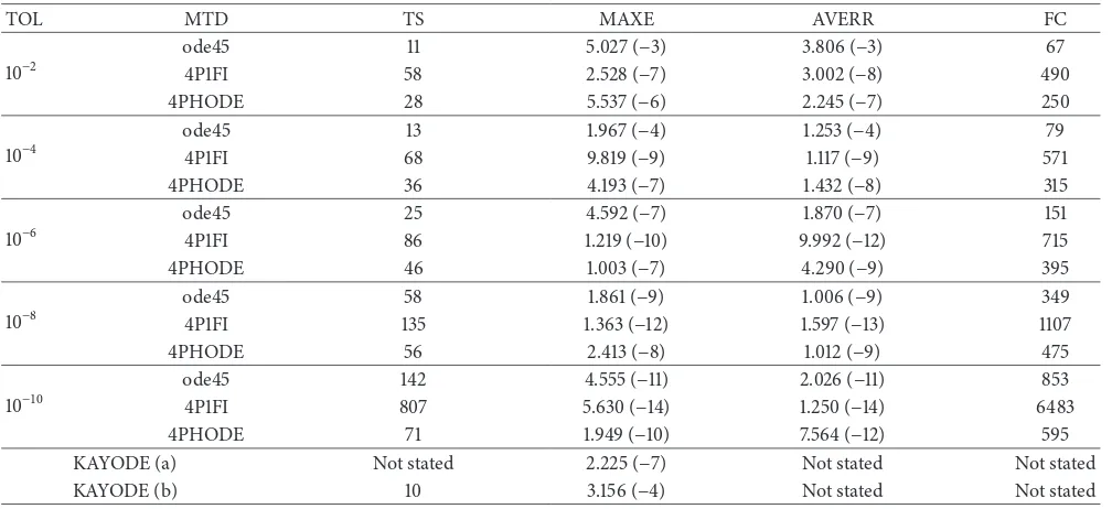
Table 2: Numerical results for solving Problem 2.

TOL MTD TS MAXE AVERR FC

10−2

ode45 11 5.027 (−3) 3.806 (−3) 67

4P1FI 58 2.528 (−7) 3.002 (−8) 490

4PHODE 28 5.537 (−6) 2.245 (−7) 250

10−4

ode45 13 1.967 (−4) 1.253 (−4) 79

4P1FI 68 9.819 (−9) 1.117 (−9) 571

4PHODE 36 4.193 (−7) 1.432 (−8) 315

10−6

ode45 25 4.592 (−7) 1.870 (−7) 151

4P1FI 86 1.219 (−10) 9.992 (−12) 715

4PHODE 46 1.003 (−7) 4.290 (−9) 395

10−8

ode45 58 1.861 (−9) 1.006 (−9) 349

4P1FI 135 1.363 (−12) 1.597 (−13) 1107

4PHODE 56 2.413 (−8) 1.012 (−9) 475

10−10

ode45 142 4.555 (−11) 2.026 (−11) 853

4P1FI 807 5.630 (−14) 1.250 (−14) 6483

4PHODE 71 1.949 (−10) 7.564 (−12) 595

KAYODE (a) Not stated 2.225 (−7) Not stated Not stated

KAYODE (b) 10 3.156 (−4) Not stated Not stated

Problem 1. Consider the following:

�(v)

= 2��− ��(iv)

− ��− 8� + (�2− 2� − 3) ��,

� ∈ [0, 2] , � (0) = 1, ��(0) = 1, ��(0) = 3, ��(0) = 1, �(iv)_{(0) = 1.} (17)

Solution is as follows:�(�) = ��+ �2. Source is [8].

Problem 2. Consider the following:

�(v)_{= 6 (2 (�}�₎3_{+ 6��}�_��_{+ �}2_��_{) , � ∈ [1, 3] , � (1) = 1, �}�_{(1) = −1, �}��_{(1) = 2, �}��_{(1) = −6, �}(iv)_{(1) = 24.} ₍₁₈₎

Solution is as follows:�(�) = 1/�. Source is [8].

5. Discussion

In this section the performances of 4PHODE, ode45, 4P1FI, KAYODE (a), and KAYODE (b) are discussed in terms of three parameters, namely, total steps taken, accuracy, and total function evaluations. It is apparent from these tables, mostly at tolerances10−2,10−4, and10−6, that 4PHODE gives better accuracy compared to ode45, whereas at tolerances

10−8and10−10, ode45 is one decimal more accurate compared to 4PHODE for both problems. As both tables show, the total steps taken by the 4PHODE reduce by nearly half to ode45 at tolerance10−10. Although, at other tolerance, ode45 requires lesser steps to compute the solution, this result may be explained by the fact that the initial step size generated by

4PHODE is extremely small in order for the method control of the accuracy. From the data in Tables 1 and 2, it is apparent that the number of function calls is likely to be related to the number of steps taken.

(8)

Comparing the results with the method proposed by KAYODE (a) and KAYODE (b), for Problem 1, 4PHODE outperformed both KAYODE (a) and KAYODE (b) in terms of accuracy and total steps taken. While, for Problem 2, KAYODE (b) has lesser total steps taken, however, 4PHODE still has superiority in terms of accuracy.

6. Conclusion

he overall performance revealed that the 4-point block method is best to be implemented in a direct integration approach as it required much less storage than the reduc-tion method while still maintaining an acceptable accuracy. Besides that, the results of this study also indicate that the developed method has better accuracy compared to the existing methods. Hence it can be said that 4PHODE is one of the alternative methods that can be used for solving ith-order ODEs.

Competing Interests

he authors declare that there are no competing interests regarding the publication of this paper.

Acknowledgments

Grateful acknowledgement is made to the Ministry of Higher Education, Malaysia, for inancial support with Grant no. RAGS/2013/FKEKK/SG04/01/B00037.

References

[1] M. T. Darvishi, S. Kheybari, and F. Khani, “A numerical solution of the Korteweg-de Vries equation by pseudospectral method

using Darvishi’s preconditionings,” Applied Mathematics and

Computation, vol. 182, no. 1, pp. 98–105, 2006.

[2] L. Jin, “Application of variational iteration method to the

ith-order KdV equation,”International Journal of Contemporary

Mathematical Sciences, vol. 3, no. 5, pp. 213–221, 2008.

[3] L. Kaur, “Generalized (G�/G)—expansion method for

gener-alized ith order KdV equation with time-dependent

coei-cients,”Mathematical Sciences Letters, vol. 3, no. 3, pp. 255–261,

2014.

[4] M. Suleiman, Z. B. Ibrahim, and A. F. N. Bin Rasedee, “Solution of higher-order ODEs using backward diference method,” Mathematical Problems in Engineering, vol. 2011, Article ID 810324, 18 pages, 2011.

[5] U. Goktas and W. Hereman, “Symbolic computation of con-served densities for systems of nonlinear evolution equations,” Journal of Symbolic Computation, vol. 24, no. 5, pp. 591–621, 1997. [6] N. Khanal, R. Sharma, J. Wu, and J.-M. Yuan, “A dual-Petrov-Galerkin method for extended ith-order Korteweg-de Vries

type equations,”Discrete and Continuous Dynamical Systems,

pp. 442–450, 2009.

[7] J. Li and Z. Qiao, “Explicit soliton solutions of the Kaup-Kupershmidt equation through the dynamical system

ap-proach,”Journal of Applied Analysis and Computation, vol. 1, no.

2, pp. 243–250, 2011.

[8] S. J. Kayode and D. O. Awoyemi, “A multiderivative Collocation

method for 5th order ordinary diferential equations,”Journal

of Mathematics and Statistics, vol. 6, no. 1, pp. 60–63, 2010. [9] S. J. Kayode, “An order seven continuous explicit method

for direct solution of general ith order ordinary diferential

equations,”International Journal of Diferential Equations and

Applications, vol. 13, no. 2, pp. 71–80, 2014.

[10] J. B. Rosser, “A Runge-Kutta for all seasons,”SIAM Review, vol.

9, no. 3, pp. 417–452, 1967.

[11] M. B. Suleiman, “Solving nonstif higher order ODEs directly

by the direct integration method,”Applied Mathematics and

Computation, vol. 33, no. 3, pp. 197–219, 1989.

[12] D. O. Awoyemi, “A new sixth-order algorithm for general

second order ordinary diferential equations,” International

Journal of Computer Mathematics, vol. 77, no. 1, pp. 117–124, 2001.

[13] S. J. Kayode, “An eicient zero-stable numerical method for

fourth-order diferential equations,” International Journal of

Mathematics and Mathematical Sciences, vol. 2008, Article ID 364021, 10 pages, 2008.

[14] B. T. Olabode and Y. Yusuph, “A new block method for

special third order ordinary diferential equations,”Journal of

Mathematics and Statistics, vol. 5, no. 3, pp. 167–170, 2009. [15] S. N. Jator and J. Li, “A self-starting linear multistep method

for a direct solution of the general second-order initial value

problem,”International Journal of Computer Mathematics, vol.

86, no. 5, pp. 827–836, 2009.

[16] N. Waeleh, Z. A. Majid, F. Ismail, and M. Suleiman, “Numerical solution of higher order ordinary diferential equations by

direct block code,”Journal of Mathematics and Statistics, vol. 8,

no. 1, pp. 77–81, 2011.

[17] L. F. Shampine and H. A. Watts, “Block implicit one-step

methods,”Mathematics of Computation, vol. 23, pp. 731–740,

1969.

[18] J. R. Cash, “Block Runge-Kutta methods for the numerical integration of initial value problems in ordinary diferential

equations. Part I. he nonstif case,”Mathematics of

Computa-tion, vol. 40, no. 161, pp. 175–191, 1983.

[19] S. N. Jator, “Solving second order initial value problems by a

hybrid multistep method without predictors,”Applied

Mathe-matics and Computation, vol. 217, no. 8, pp. 4036–4046, 2010. [20] N. Waeleh, Z. A. Majid, and F. Ismail, “A new algorithm for

solving higher order IVPs of ODEs,” Applied Mathematical

Sciences, vol. 5, no. 53–56, pp. 2795–2805, 2011.

[21] J. Vigo-Aguiar and H. Ramos, “Variable stepsize

implemen-tation of multistep methods for y��=f(x, y, y�),” Journal of

Computational and Applied Mathematics, vol. 192, no. 1, pp. 114– 131, 2006.

[22] Z. A. Majid, N. A. Azmi, M. Suleiman, and Z. B. Ibrahaim, “Solv-ing directly general third order ordinary diferential equations

using two-point four step block method,”Sains Malaysiana, vol.

41, no. 5, pp. 623–632, 2012.

[23] J. D. Lambert,Computational Methods in Ordinary Diferential

Equations, John Wiley & Sons, London, UK, 1973.

[24] S. Ola Fatunla, “Block methods for second order ODEs,” International Journal of Computer Mathematics, vol. 41, no. 1-2, pp. 55–63, 1991.

[25] Z. A. Majid and M. B. Suleiman, “Implementation of four-point fully implicit block method for solving ordinary diferential

equations,”Applied Mathematics and Computation, vol. 184, no.

(9)

Submit your manuscripts at

http://www.hindawi.com

Hindawi Publishing Corporation

http://www.hindawi.com Volume 2014

Mathematics

Journal of

Mathematical Problems in Engineering

Hindawi Publishing Corporation http://www.hindawi.com

Differential Equations International Journal of

Volume 2014

Mathematical PhysicsAdvances in

Complex Analysis

Journal of

Optimization

Journal of

Combinatorics

http://www.hindawi.com Volume 2014 International Journal of

Journal of

Function Spaces

Abstract and Applied Analysis

International Journal of Mathematics and Mathematical Sciences

Hindawi Publishing Corporation http://www.hindawi.com Volume 2014

The Scientiic

World Journal

Discrete Dynamics in Nature and Society

Discrete Mathematics

Journal of

http://www.hindawi.com Volume 2014 Hindawi Publishing Corporation