7-6-2010
he Requirement of a Positive Deinite Covariance
Matrix of Security Returns for Mean-Variance
Portfolio Analysis: A Pedagogic Illustration
Clarence C. Y. Kwan
McMaster University, [email protected]
Follow this and additional works at:
htp://epublications.bond.edu.au/ejsie
his work is licensed under a
Creative Commons Atribution-Noncommercial-No Derivative Works
4.0 License
.
his Regular Article is brought to you by the Bond Business School atePublications@bond. It has been accepted for inclusion in Spreadsheets in Education (eJSiE) by an authorized administrator of ePublications@bond. For more information, please contactBond University's Repository Coordinator.
Recommended Citation
Kwan, Clarence C. Y. (2010) he Requirement of a Positive Deinite Covariance Matrix of Security Returns for Mean-Variance Portfolio Analysis: A Pedagogic Illustration,Spreadsheets in Education (eJSiE): Vol. 4: Iss. 1, Article 4.
his study considers, from a pedagogic perspective, a crucial requirement for the covariance matrix of security returns in mean-variance portfolio analysis. Although the requirement that the covariance matrix be positive deinite is fundamental in modern inance, it has not received any atention in standard investment textbooks. Being unaware of the requirement could cause confusion for students over some strange portfolio results that are based on seemingly reasonable input parameters. his study considers the requirement both informally and analytically. Electronic spreadsheet tools for constrained optimization and basic matrix operations are utilized to illustrate the various concepts involved.
Keywords
Mean-Variance Portfolio Analysis, Positive Deinite Covariance Matrix, Excel Illustration
Distribution License
The Requirement of a Positive De…nite Covariance Matrix
of Security Returns for Mean-Variance Portfolio Analysis:
A Pedagogic Illustration
Clarence C.Y. Kwan DeGroote School of Business
McMaster University Hamilton, Ontario L8S 4M4
Canada
E-mail: [email protected]
July 2010
Abstract
This study considers, from a pedagogic perspective, a crucial requirement for the covariance matrix of security returns in mean-variance portfolio analysis. Although the requirement that the covariance matrix be positive de…nite is fundamental in modern …nance, it has not received any attention in standard investment textbooks. Being unaware of the requirement could cause confusion for students over some strange portfolio results that are based on seemingly reasonable input parameters. This study considers the requirement both informally and analytically. Electronic spreadsheet tools for constrained optimization and basic matrix operations are used to illustrate the various concepts involved.
Submitted May 2010, revised and accepted July 2010.
Key words: mean-variance portfolio analysis, positive de…nite covariance matrix,
Excel spreadsheet illustration
1
Introduction
This study considers, from a pedagogic perspective, a crucial analytical requirement on input parameters for mean-variance portfolio analysis. Being traditionally considered to be beyond the scope of the standard …nance curriculum, the requirement is seldom brought to the attention of students, even in advanced portfolio investment courses. As a result, there is an undesirable gap between what is viewed as fundamental in the academic …nance literature and what students learn in investment courses. Being unaware of the requirement could lead to confusion over some strange portfolio results that are based on seemingly reasonable input parameters.
Speci…cally, the requirement is that the covariance matrix of security returns, which contains all variances and covariances of returns of the securities considered, be positive
de…nite.1 In the context of portfolio investments under the assumption of frictionless
short sales, the covariance matrix is positive semide…nite if the variance of portfolio re-turns is always non-negative, regardless of how investment funds are allocated among
the securities considered.2 If the portfolio variance is always strictly positive, the
covari-ance matrix is also positive de…nite. A positive de…nite covaricovari-ance matrix is invertible; however, a covariance matrix that is positive semide…nite but not positive de…nite is not invertible.
At …rst glance, as the variance of a random variable, by de…nition, cannot be negative, the attainment of a positive de…nite covariance matrix seems to be assured if individual securities or their combinations that can lead to risk-free investments are excluded from portfolio consideration. As shown in Appendix A, the sample covariance matrix — the covariance matrix estimated from a sample of past return observations — is always positive semide…nite. Once the various situations causing the sample covariance matrix to be non-invertible are ruled out, the positive de…niteness requirement will be satis…ed. Then, why is the requirement still a relevant issue to consider? That is because the
variance of a linear combination of some random variables, as expresseddirectly in terms
of the variances and covariances of these variables, can be negative if not all individual variances and covariances correspond to their sample estimates. Here are some speci…c examples:
In classroom settings, input parameters for numerical illustrations of portfolio analy-sis are often generated arti…cially. Although the covariance matrix for more than two securities thus generated is invertible, with the implied correlations of returns between
di¤erent securities being always in the permissible range of 1to1;whether it is positive
de…nite is not immediately obvious. In practical settings, security analysts’ insights are often required to revise the sample estimates of input parameters for portfolio analysis in order to recognize changes in the economic environment. Likewise, for a high-dimensional portfolio selection problem, if the covariance matrix is estimated with insu¢cient
ob-1The requirement is explicitly stated in Merton (1972), Roll (1977), and Jobson and Korkie (1989),
among others.
2Under the assumption of frictionless short sales, if an investor short sells a security, the investor not
servations (for concerns about outdated return data from a long sample period), some
matrix elements will have to be revised to make the resulting matrix invertible.3 In
ei-ther case, it is not immediately obvious wheei-ther the resulting matrix is positive de…nite. Further, if estimation of the covariance matrix is based on models that can accommo-date time-varying volatility of security returns, the positive de…niteness of the resulting covariance matrix may not be assured.
In this study, we consider the positive de…niteness requirement …rst informally and then analytically, in order to accommodate di¤erent pedagogic approaches — which correspond to di¤erent levels of analytical rigor — in the delivery of the mean-variance
portfolio concepts to the classroom.4 In an informal approach, we illustrate with a
three-security case that having all correlations of three-security returns in the permissible range of
1to1alone does not ensure the validity of the covariance matrix. Speci…cally, by using
Microsoft ExcelT M; we compute the covariances and correlations of returns of various
portfolios. Further, we useSolver, a numerical tool in Excel, to search for the allocation
of investment funds (under the assumption of frictionless short sales) that corresponds to the lowest variance of portfolio returns. If it turns out that any correlations of portfolio returns are outside the permissible range or the lowest variance is negative, then the covariance matrix in question cannot be acceptable.
In our analytical approach to consider the positive de…niteness requirement, the alge-braic and statistical tools involved are con…ned to those known to most business students. By using a basic portfolio selection model, in which frictionless short sales are assumed, we can directly reach the portfolio solution in terms of the input parameters provided. We can also address the issue of positive de…niteness without being encumbered by the algorithmic details that are often associated with solution methods for more sophisti-cated portfolio selection models. For ease of exposition, matrix notation is used. The required matrix operations, which are basic, can easily be performed on spreadsheets.
3There are various empirical approaches to ensure the invertibility of a covariance matrix, even if there
are insu¢cient observations for its estimation. A simple approach is to impose a particular covariance structure. In the case of the constant correlation model, for example, all correlations of security returns are characterized to be the same. In such a case, the estimated covariances are based on the individual sample variances and a common correlation. The use of the average of all sample correlations for the securities considered as the common correlation will ensure that the resulting covariance matrix be positive de…nite. [See Kwan (2006) for some analytical properties of the constant correlation model.] A more sophisticated approach to ensure positive de…niteness is shrinkage estimation, which takes a weighted average of the sample covariance matrix and a structured matrix. [See Ledoit and Wolf (2004) and Kwan (2008) for analytical details of the shrinkage approach in which the structured matrix is based on the constant correlation model.]
4In advanced investment courses, it is also useful to justify analytically the mean-variance approach,
They include matrix transposition, addition, multiplication, and inversion, as well as …nding the determinant. As this study is intended to be self-contained for pedagogic purposes, the analytical materials involved are derived. Some proofs are provided in footnotes or appendices, in order to avoid digressions.
The rest of this study is organized as follows: Section 2 provides a two-security ex-position of basic portfolio concepts. An extension to a three-security case is presented in Section 3. An Excel example there illustrates the need for addressing the positive def-initeness issue. Section 4 presents a basic portfolio selection model. As the covariance matrix must be invertible for the model to provide any portfolio allocation results, situ-ations leading to its non-invertibility are …rst identi…ed in Section 5. The central theme of Section 5 is that, for the portfolio allocation results to be meaningful, the covariance matrix must be positive de…nite. It implications are also considered there. With the aid of an Excel example, Section 6 illustrates some consequences for violating the positive de…niteness requirement. Finally, Section 7 provides some concluding remarks.
2
Portfolio concepts based on two securities
In introductory …nance courses, the delivery of mean-variance portfolio concepts typically starts with a two-security case, where the security with a higher expected return also
has a higher variance of returns. With the random returns of the two securities beingR1
andR2 and their expected returns being 1 and 2;each of the two variances of returns,
labeled as 2
1 and 2
2;is the expected value of the squared deviation of the corresponding
random return from its mean. The covariance of returns of R1 and R2; labeled as 12;
is the expected value of (R1 1)(R2 2): The correlation of returns 12; de…ned as
12=( 1 2); is always in the range of 1 to 1: It is implicit that 11 = 12; 22 = 22;
12= 21; 12= 21; 11= 11=( 1 1) = 1;and 22= 22=( 2 2) = 1:
Suppose that a portfolio p is formed, with the proportions of investment funds as
allocated to the two securities — the portfolio weights — being x1 and x2 = 1 x1:
Under the assumption of frictionless short sales, each portfolio weight can be of either
sign. The variance of portfolio returns, labeled as 2
p;is the expected value of(Rp p)2;
Equations (2) and (4), when combined to eliminate the portfolio weights, will allow p
are perfectly correlated (i.e., 12= 1);the relationship between p and p is linear or
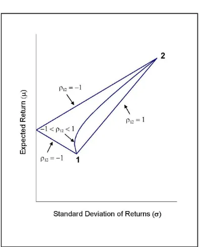
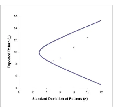
piecewise linear; otherwise, it is nonlinear. Figure 1 shows some graphs on the ( ; )
-plane — where standard deviation of returns and expected return are the horizontal
and vertical axes, respectively — that are commonly used in introductory …nance courses for describing the risk-return trade-o¤ from investing in two risky securities without short sales.
These graphs reveal some basic portfolio concepts. Speci…cally, if 12= 1;as the
risk-return trade-o¤ in portfolio investments is captured by the line joining points ( 1; 1)
and ( 2; 2); there is no diversi…cation e¤ect. If 12 <1 instead, portfolio investments
in the two securities will lead to risk reductions for any expected return requirements
(as compared to the case where 12 = 1):The lower the correlation, the greater is the
risk-reduction e¤ect. If 12= 1;a risk-free portfolio can be reached. Notice that, under
the assumption of frictionless short sales, the line joining points ( 1; 1)and( 2; 2) for
the case where 12 = 1 can be extended to reach its -intercept; that is, if 12 = 1; a
risk-free portfolio can also be reached.
If 1 < 12 <1;no investments in the two securities can completely eliminate the
portfolio risk. To see this, let us rewrite equation (4) as
2
by completing the square. With 1 2
12 being positive, there are no portfolio weights of
either sign that can result in 2
p being zero or negative.
In linear algebra, it is known as Sylvester’s Criterion that a real symmetric matrix is positive de…nite if and only if all of its leading principal minors are positive. For an
n n matrix, there arenleading principal minors, each of which is the determinant of
the submatrix containing the …rst krows and the …rst k columns, fork= 1;2; : : : ; n:A
proof of this matrix property is provided in Appendix B. The 2 2 covariance matrix
11 12
21 22
under the condition of 1 < 12 < 1 is positive de…nite because both
of its leading principal minors, 11 (= 21) and 11 22 21 12 [= 21
2 2(1
2
12)]; are positive. Thus, in a two-security case, if the returns of the two securities are not perfectly correlated, the positive de…niteness requirement is automatically satis…ed.
3
A three-security illustration of the positive de…niteness
requirement
Depending on the …nance courses involved, extensions to portfolio investments in more than two risky securities can di¤er considerably. Regardless of the pedagogic approach
that is followed, the e¢cient frontier on the ( ; )-plane, which captures the best
A common message from the various pedagogic approaches is that, as long as the risky securities considered are less than perfectly, positively correlated, there will be portfolio diversi…cation e¤ects. To ensure the attainment of a meaningful e¢cient fron-tier, however, a relevant question now is whether there is any other requirement for the covariance matrix beyond having all correlations of security returns in the permissible
range of 1 to 1: As investment textbooks are silent on the issue, we illustrate below
with a simple three-security example that a further requirement is warranted.
To facilitate the illustration, let R1; R2; R3; 1; 2; and 3 be the random and
expected returns of the three-risky securities considered. The three variances ( 2
1 = 11; 2
2 = 22; and 32 = 33) and the six covariances ( 12 = 21; 13 = 31; and 23 = 32)
of security returns can be arranged as elements of a3 3 covariance matrix. With each
element (i; j) being ij; which is the same as ji; for i; j = 1;2; and 3;the covariance
matrix is symmetric. A 3 3 correlation matrix can be inferred directly from the
covariance matrix.
We now allocate investment funds in two di¤erent ways, with the corresponding
portfolios labeled as pand q: For portfolio p;letx1; x2;and x3 be the portfolio weights
satisfying the condition of x1 +x2 +x3 = 1: The random return and the expected
return of the portfolio are Rp = x1R1+x2R2 +x3R3 and p = x1 1 +x2 2 +x3 3;
respectively. The variance of returns of the portfolio, 2
p;which is the expected value of
(Rp p)2 = [x1(R1 1) +x2(R2 2) +x3(R3 3)]2;can be expressed as the sum
q;can be computed in an analogous manner. The covariance of returns of
portfolios p and q; labeled as pq; is the expected value of (Rp p)(Rq q): When
expressed in terms of the variances and covariances of the individual securities, pq
is the sum of nine terms of the form xiyj ij; for i; j = 1;2; and 3; that is, pq =
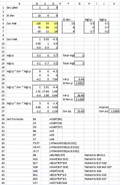
Figure 2 shows an Excel worksheet for a three-security case, where all returns are mea-sured in percentage terms. The variances and covariances of returns provided for the
example consist of 2
to symmetry, 21; 31; and 32 can be inferred directly. The 3 3 covariance matrix
of returns is shown in cellsB5:D7 of the worksheet. The implied correlations of returns,
as shown in cells B9:D11, are all in the permissible range of 1 to 1: Notice that cell
formulas are listed at the bottom of Figure 2. Likewise, whenever an Excel worksheet is displayed in any of the subsequent …gures, cell formulas are listed as well.
To see whether having all pairwise correlations in the permissible range alone is suf-…cient to ensure the validity of the covariance matrix, we have attempted di¤erent
allo-cations of investment funds for portfoliospandq:In each case, we have checked whether
the correlation of portfolio returns, de…ned as pq = pq=( p q); is in the permissible
cellsB13:D13 and B15:D15. Whenever there are changes in these portfolio weights, the
corresponding computational results are automatically updated in the worksheet. The results in Figure 2 are from one of the many sets of portfolio weights that
invalidate the covariance matrix in cells B5:D7. Speci…cally, for x1 = 0:3; x2 = 0;
x3 = 0:7; y1 = 0:1; y2 = 0:7; and y3 = 0:2; the computed values of xixj ij; yiyj ij;
and xiyj ij; for i; j = 1;2;3; are displayed in cells B17:D19, B21:D23, and B25:D27,
respectively. Summing the individual 3 3 blocks gives us 2
p = 8:44; q2 = 26:46;and pq = 15:45;as shown in cells G19,G23, and G27, respectively. The implied correlation pq = 1:0339;as shown in cellK27, is outside the permissible range, thus indicating that
the covariance matrix in question is unacceptable.
This example points out that there must be a requirement for the covariance matrix of security returns in addition to, or encompassing, the obvious requirement that all
pairwise correlations be in the permissible range of 1 to 1: The requirement is that
the covariance matrix be positive de…nite. In the context of portfolio investments under the assumption of frictionless short sales, the requirement amounts to the variance of portfolio returns being always strictly positive, regardless of how investment funds are allocated among the risky securities considered. A simple way to …nd out whether the
3 3covariance matrix is positive de…nite is by searching, with the numerical toolSolver
in Excel, for the set of portfolio weights that minimizes the variance of portfolio returns. If the numerical search produces a strictly positive variance of portfolio returns, the covariance matrix is positive de…nite; otherwise, it is not.
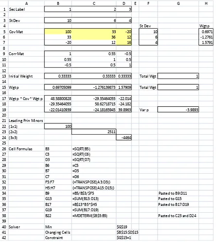
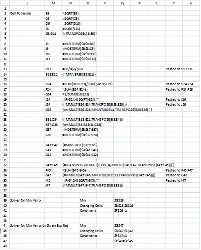
Figure 3 shows the Solver results. Initially, with the contents of cells B13:D13 —
which provide equal portfolio weights (of1=3 each) for the three securities — copied to
cellsB15:D15, the corresponding variance of portfolio returns is displayed in cellG19, by
following the same computational steps for portfolio p in Figure 2. The initial results
are not shown in Figure 3, as any changes in cellsB15:D15will automatically allow cell
G19to be updated. By using Solver, we minimize the target cell G19, by changing the
portfolio weights in cells B15:D15, subject to the constraint that cell G15, the sum of
the portfolio weights, be equal to 1: As the lowest variance from the numerical search,
displayed in cell G19 is 3:9893; is a negative number, the covariance matrix in cells
B5:D7is not positive de…nite.
An alternative way to use Excel to …nd out whether the covariance matrix is positive de…nite is by checking the signs of all leading principal minors of the covariance matrix. In a three-security case, the three leading principal minors are the determinants of the
h h matrices consisting of the …rst h columns and the …rst h rows of the covariance
matrix, for h = 1; 2; and 3: As shown in cells B22, C23, and D24, the three leading
principal minors are100;2511;and 4464;respectively. With the presence of a negative
number here, the 3 3covariance matrix is not positive de…nite and is thus invalid.
As the validity of a given covariance matrix as part of the input parameters for portfolio analysis is not readily noticeable, the above example illustrates the importance of verifying its positive de…niteness. A positive de…nite covariance matrix can sometimes di¤er from a non-positive de…nite case in just a few matrix elements. For example, if we
A B C D E F G H I J K
26 6.93 0 5.88 Implied
27 -1.2 0 2.24 Cov pq 15.45 Corr pq 1.0339 28
29 Cell Formulas B3 =SQRT(B5)
30 C3 =SQRT(C6)
38 B9 =B5/B$3/$F5 Pasted to B9:D11 39 G13 =SUM(B13:D13) Pasted to G15 40 B17 =B$13*B5*$H5 Pasted to B17:D19 41 G19 =SUM(B17:D19) Pasted to G23 and G27 42 G20 =SQRT(G19) Pasted to G24
43 B21 =B$15*B5*$J5 Pasted to B21:D23 44 B25 =B$13*B5*$J5 Pasted to B25:D27 45 K27 =G27/G20/G24
A B C D E F G H
13 Initial Weight 0.33333 0.33333 0.33333 Total Wgt 1
14
15 Wgt p 0.69705099 -1.276139873 1.57909 Total Wgt 1
16
17 Wgt p * Cov * Wgt p 48.58800828 -29.35464055 -22.014
18 -29.35464055 58.62718715 -24.182
19 -22.01410939 -24.18165945 39.8963 Var p -3.9893
20
26 Cell Formulas B3 =SQRT(B5)
27 C3 =SQRT(C6)
34 B9 =B5/B$3/$F5 Pasted to B9:D11
35 G13 =SUM(B13:D13) Pasted to G15
36 B17 =B$13*B5*$H5 Pasted to B17:D19
37 G19 =SUM(B17:D19)
38 B22 =MDETERM($B$5:B5) Pasted to C23 and D24
39
40 Solver Min $G$19
41 Changing Cells $B$15:$D$15
42 Constraint $G$15=1
matrix unchanged, the same computations for the worksheets in Figures 2 and 3 will con…rm that the revised covariance matrix is positive de…nite.
Speci…cally, regardless of how investment funds are allocated in portfolios p and q;
the implied correlations of portfolio returns, as displayed in cellK27of the worksheet in
Figure 2, are always in the permissible range. The Solver result of the lowest possible
portfolio variance, as displayed in cellG19of the worksheet in Figure 3, becomes7:2995;
a positive number instead. Further, the three leading principal minors, as displayed in
cells B22, C23, and D24 of the same worksheet are 100; 2511; and 11088; respectively;
that is, they are all positive.
4
A basic portfolio selection model
The above Excel example illustrates that, for the portfolio solution to be meaningful, the covariance matrix involved must be positive de…nite. However, this being an illustration, the positive de…niteness requirement still has to be justi…ed properly. The task requires the use of a portfolio selection model. Following Roll (1977), we minimize the variance
of portfolio returns, for a given set of n risky securities, subject to an expected return
requirement. Under the assumption of frictionless short sales, if a portfoliop is formed,
its expected return and variance of returns are
p =
respectively, satisfying the condition ofPni=1xi = 1:In matrix notation, let andxben
-element column vectors of expected returns and portfolio weights, with the corresponding
elements being i and xi; for i = 1;2; : : : ; n: Let V be a symmetric n n covariance
matrix of returns, with its element (i; j)being ij;fori; j= 1;2; : : : ; n:Let also be an
n-element column vector where each element is 1: Then, equations (6) and (7) can be
written more compactly as p =x0 and p2=x0V x;withx0 = 1:
For a predetermined p;the Lagrangean is
L=x0V x (x0 p) (x0 1); (8)
where the portfolio weight vector x and the Lagrange multipliers and are decision
variables.5 It is implicit that the elements of are not all equal; otherwise, as all
portfolios based on the n securities will have the same expected return, the use of a
predetermined p that di¤ers from this expected return will inevitably fail to provide
any portfolio allocation results. Minimizing Lleads to
x=V 1M(M0V 1M) 1rp; (9)
5See Kwan (2007) for an equivalent formulation of the same portfolio selection problem and for an
where M = is an n 2 matrix and rp = p 1 0 is a 2-element column
vector.6 The variance of returns of the minimum variance portfolio (for a predetermined
p) is
2
p =x0V x=rp0(M0V
1
M) 1rp: (10)
By repeating the computations based on equation (9) for di¤erent values of p;we can
establish a family of minimum variance portfolios. The least risky portfolio of the family is called the global minimum variance portfolio. Such a portfolio can also be reached
by minimizing x0V x subject only to x0 = 1:Similar to the derivation of equation (9),
minimizing the LagrangeanL=x0V x (x0 1)leads to
xo=V 1 ( 0V 1 ) 1: (11)
Here, the vector of portfolio weights, x; has been labeled as xo instead for notational
clarity. The expected return and the variance of returns of the global minimum variance portfolio are
o= 0xo = 0V 1 ( 0V 1 ) 1 (12)
and o2=xo0V xo= ( 0V 1
) 1; (13)
respectively.
As equation (13) shows, the variance of returns of the global minimum variance portfolio is the reciprocal of the sum of all elements of the inverse of the covariance matrix. The proportion of investment funds for each security in this portfolio, according to equation (11), is the sum of all elements of the corresponding row of the inverse of the covariance matrix, divided by the sum of all elements of the same inverse matrix. Thus, the sum of portfolio weights being unity is assured.
5
The positive de…niteness requirement and its
implica-tions
From an analytical perspective, equations (9)-(13) are results of the …rst-order conditions for optimization. Whether such results actually correspond to variance minimization as intended, rather than variance maximization or the presence of saddle points, still
requires con…rmation. Of interest, therefore, is whether the input parameters andV
are required to satisfy some speci…c conditions in order to ensure variance minimization. As an initial step in the search of conditions on the input parameters for equations (9)-(13) to work properly, we must ensure that the covariance matrix be invertible. Noting that the invertibility of the covariance matrix requires its determinant to be non-zero, we must rule out the following three situations. First, if a security considered is
6To derive equation (9), we use@L=@x= 2V x =0;where0is ann-element column vector
of zeros. This equation can be rewritten asx= 1 2V
risk-free, it will have a zero variance of returns and zero covariances of returns with all other securities considered; this situation will produce a row (column) of zeros in the covariance matrix. Second, if the random return of a security is perfectly correlated with that of another security considered, two rows (columns) of the covariance matrix will be proportional to each other. Third, if the random return of a security is a linear combination of the random returns of some other securities considered, a row (column) of the covariance matrix can be replicated exactly by combining other rows (columns). In each situation, the covariance matrix is non-invertible, as the corresponding determinant is zero. The above three situations arising from sample estimates of the covariance matrix are considered in more detail in Appendix A.
Students in portfolio investment courses, most likely, are made aware of the above three situations and their implications. The presence of a risk-free security transforms the portfolio selection problem into a two-part problem, with the …rst part pertaining to the selection of a portfolio based only on the risky securities and the second part pertaining to the allocation of investment funds between the risk-free security and the risky portfolio. In the remaining two situations, the contribution of a security to the risk-return trade-o¤ of the portfolio can be replicated exactly by that of another security or a combination of other securities. Thus, the portfolio selection results will no longer be unique, and equations (9)-(13) will fail to perform their intended tasks.
With the above three situations ruled out, we now show that, for equations (9)-(13) to work properly, the covariance matrix must be positive de…nite. Indeed, if the covariance matrix is positive de…nite, the above three situations will automatically be ruled out, and
these equations will work as intended. In the language of matrix algebra, ann nmatrix
V is positive semide…nite if x0V x; which is a scalar, is always non-negative for any n
-element column vector x: It is also positive de…nite if x0V x is strictly positive for any
non-zero vector x: In the context of portfolio analysis, V is the covariance matrix and
x is the portfolio weight vector. As it will soon be clear, with the positive de…niteness
requirement satis…ed, the invertibility ofV;M0V 1M;and 0V 1
is assured. However, the converse is not true; the invertibility of these matrices does not ensure that the covariance matrix be positive de…nite.
We now turn our attention to the condition for a minimized Lagrangean in the basic
portfolio selection model. In that model, we seek to minimize the Lagrangean L in
equation (8) with the portfolio weights x1; x2; : : : ; xn and the Lagrange multipliers
and being the decision variables. Now, for ease of exposition, let us treat and as
xn+1 and xn+2; respectively. As the Lagrangean Lis a quadratic function of the n+ 2
decision variables, its partial derivatives beyond the second order are all zeros. Then,
with L being the Lagrangean as evaluated atx1 =x1; x2 =x2; : : : ; xn+2 =xn+2; for
which its …rst partial derivative with respect to each of the n+ 2 variables is set to be
zero, we can express L by means of a second-order Taylor expansion. That is, we can
where each second partial derivative is evaluated atx1=x1; x2 =x2; : : : ; xn+2 =xn+2:7
The(n+ 2) (n+ 2)symmetric matrix consisting of the above second partial
deriva-tives is commonly called the bordered Hessian. In such a matrix, we have@2
L=(@xi@xj) =
0: With4x being arbitrary, we con…rm that minimization of the Lagrangean requires
the covariance matrix to be positive de…nite.8
The sub-sections below show various implications of the covariance matrix being positive de…nite, along with some cautionary notes.
5.1 The inverse of the covariance matrix and the global minimum vari-ance portfolio
If the covariance matrix V is positive de…nite, so is V 1: The reason is that, as V is
invertible and asx0V xis positive for any non-zero column vector x;
x0V x=x0V(V 1V)x=(V x)0V 1
(V x) (16)
is also positive. WithV x being an arbitrary column vector and (V x)0 being its
trans-pose, the positive de…niteness of V 1 is assured. If an invertible V is not positive
de…nite, a non-zero column vector x corresponding to x0V x being non-positive must
exist. For such a vectorx; we have a corresponding column vectorV x:Then, in view
of equation (16),V 1 is also not positive de…nite.
Now, suppose thatV is invertible but its positive de…niteness has not been con…rmed.
For V 1 to be positive de…nite, it must not have any negative diagonal elements. To
verify this requirement, suppose instead that V 1 has at least a negative diagonal
el-ement, with element (i; i) being negative. Let c be an n-element column vector with
7For students who are unfamiliar with multivariate Taylor series, an explanation of equation (14) is
necessary. The idea is similar to the expansion of a quadratic functionL(x): In this univariate case, we haveL(x) =L(x ) + (x x )L0(x ) +1
2(x x )
2
L00(x );with the derivatives evaluated atx=x : To extend to a multivariate case, we must account for all second derivatives ofL;that is,@2L=(@x
i@xj);for alli; j: This is captured by the terms under the double summation on the right hand side of equation (14).
8The above proof encompasses, as a special case, the Lagrangian that is intended for the global
minimum variance portfolio. In this special case with n+ 1 decision variables, the only Lagrange multiplier, ;can be treated asxn+1:Equation (15) can be rewritten analogously. Forx1; x2; : : : ; xn+1
elementibeing its only non-zero element. In such a case,c0V 1cis negative.9 AsV 1
is not positive de…nite, its inverse — which is V — cannot be positive de…nite. The
implication is that, if the inverse of the covariance matrix has any negative diagonal elements, the covariance matrix itself cannot be positive de…nite.
The positive de…niteness of V; which implies the same for V 1; ensures that the
scalar 0V 1
be positive. IfV is positive de…nite, then, with( 0V 1
) 1being positive,
equations (11)-(13) do provide portfolio allocation results for the global minimum
vari-ance portfolio as intended. However, without …rst con…rming thatV is positive de…nite,
we cannot con…rm the validity of the results from these equations even if ( 0V 1
) 1 turns out to be positive.
What is crucial here is that, although the set of portfolio weights from equation
(11) allows us to compute the corresponding variance of portfolio returns as( 0V 1
) 1; whether this variance is the lowest possible variance still depends on the positive
def-initeness of V: If V is not positive de…nite, the set of portfolio weights from equation
(11) does not give us a minimum of the Lagrangean L;what we get can be a maximum
or a saddle point instead.
5.2 The inverse of a 2 2 matrix in the basic portfolio selection model and minimum variance portfolios
The invertibility of the 2 2 matrixM0V 1M in equations (9) and (10) requires that
its determinant — labeled askhere — be non-zero. As the elements (1;1);(1;2);(2;1); invertible, we draw on the matrix property that a symmetric positive de…nite matrix can be written as a product of a square matrix and its transpose. The proof of this matrix property is provided in Appendix C.
Speci…cally, withV 1 being symmetric and positive de…nite, we can write V 1 =
LL0;whereL is ann nmatrix. It follows that
whereai is element iof the column vectorL0 :Likewise, we can write
Drawing on Cauchy-Schwarz inequality, we have
can be ruled out. A simple algebraic proof of Cauchy-Schwarz inequality is provided in Appendix D. As it is implicit in the model formulation in Section 4 that the elements
of are not all equal, strict inequality is assured; that is, k is strictly positive and,
accordingly,M0V 1
M is invertible.
The positive de…niteness of V ensures that the two leading principal minors of the
2 2 matrix M0V 1M — which are 0V 1
and k — are both positive. That is,
ifV is positive de…nite, so are M0V 1
M and (M0V 1
M) 1:Then, regardless of the
value of p in the2-element column vectorrp in equations (9) and (10), these equations
will always provide minimum variance portfolios, all with positive variances of portfolio
returns, as intended. However, if V is invertible but not positive de…nite, the 2 2
matrixM0V 1
M based on some given input parameters and V can still be positive
de…nite, as indicated by both 0V 1
and k being positive. In such a case, although
equation (10) will still provide positive variances of portfolio returns for all values of p;
the results are invalid, as they do not correspond to minimization of the LagrangeanL:
Therefore, it is important to con…rm the positive de…niteness ofV before accepting the
results from equations (9) and (10).
5.3 Graphs of minimum variance portfolios on the ( ; )-plane
Let us label elements(1;1);(1;2);and(2;2)of the symmetric matrix(M0V 1 we can write equation (10) as
2
p =
2
p+ 2 p+ ; (22)
which, by completing the square, becomes
2
andkare positive. Accordingly, and 2
are also positive. Thus, with( 2
)= being positive, equation (23) is a hyperbola with
a horizontal transverse axis on the( ; )-plane. The centre of the hyperbola is the point
(0; = ) on the ( ; )-plane and its vertices are the points p( 2)= ; = :
With = = o and ( 2)= = o2; representing the expected return and the
variance of returns of the global minimum variance portfolio, respectively, equation (23) can also be written as
2
p = ( p o)
2
+ 2
By de…nition, standard deviations are never negative. Thus, the relevant branch of
the hyperbola is the one where p>0:With the transverse axis of the hyperbola being
horizontal, this branch can accommodate all values of p;that is, there will not be any
value of p that can lead to a negative 2p:The e¢cient frontier is the upper half of this
branch, starting from the global minimum variance portfolio. It is a concave curve on
the ( ; )-plane, as indicated by d p=d p >0 and d2 p=d 2p <0:This characterization
of the e¢cient frontier is what students learn in investment courses.
However, ifV is not positive de…nite, the graph of equation (23) on the ( ; )-plane
can be any conic section, depending on the signs of and 2
:More speci…cally, we
have the following potential cases:
1. If both and 2
; as computed from the input parameters and V; are
positive, the graph is also a hyperbola with the same characteristics as described above.
2. If is positive, but 2
is negative instead, the resulting hyperbola will have the -axis as its transverse axis.
3. If both and 2 are negative, the graph is an ellipse.10
4. If = 0; equation (22) reduces to 2
= 2 + ; which is a parabola with the
-axis being its axis of symmetry.11
Among the four cases here, only the …rst case provides positive portfolio variances
for all predetermined values of p: In the remaining three cases, if the predetermined
p does not have a corresponding p on the graph, a negative p2 will be produced. For
example, in the second case, if p is set at values in the gap between the two vertices
of the hyperbola, there cannot be any corresponding real values of p:Obviously, none
of graphs of risk-return trade-o¤ for these three cases resemble what students learn in investment courses.
Then, is the …rst case above acceptable? Although it provides a seemingly reasonable
graph on the ( ; )-plane, with d p=d p > 0 and d2 p=d p2 < 0 for all portfolios with
expected returns greater than o;the graph does not correspond to the e¢cient frontier.
The point ( o; o) does not even correspond to the global minimum variance portfolio.
The reason is that none of the portfolios on the graph are results of minimization of the
LagrangeanL;instead, they correspond to saddle points ofL as a function of then+ 2
decision variables,x1; x2; : : : ; xn; ;and :
1 0If is negative and 2
is positive instead, equation (23) cannot be graphed on the( ; )-plane.
1 1For equation (9) to produce any portfolio allocation results,M0V 1
M must be invertible. Thus, the determinant of M0V 1
M cannot be zero. The determinant of(M0V 1
M) 1
;which is 2
;
is the reciprocal of the determinant ofM0V 1
M: Thus, with 2
5.4 Implied correlations of returns
Satisfaction of the positive de…niteness requirement for the n n matrix ensures that
its …rst two leading principal minors be positive. That is, we must have 1 < 12<1:
There aren!ways to label thensecurities as1;2; : : : ; nand to arrange the corresponding
variances and covariances of security returns in ann nmatrix. As any pair of securities
can be labeled as securities 1 and 2;the positive de…niteness requirement ensures that
1 < ij < 1; for all i 6= j: However, as illustrated in the Excel example earlier, the
converse is not true; having all pairwise correlations in the permissible range does not imply a positive de…nite covariance matrix. This explains why a covariance matrix where all implied pairwise correlations of returns are in the permissible range can still give us strange portfolio results.
As 2 is the determinant of(M0V 1
M) 1;its being positive ensures that the
correlation of returns between any two minimum variance portfolios be in the range of
1to1:To see this, let pq be the covariance of returns between two arbitrary minimum
variance portfolios p and q with expected returns p and q; respectively. Given the
corresponding portfolio weight vectorsxandy;the covariance is pq =x0V y:According
to equation (9), we have
x0V y=r0(M0V 1
can also be written as
A= p 1
q 1 (
M0V 1
M) 1 p q
1 1 : (27)
Thus, the determinant ofAis the product of the determinants of the three2 2matrices
on the right hand side of equation (27); that is,
pp qq qp pq= ( p q)2( 2): (28)
ForV being positive de…nite, noting that 2
is positive, we have ( pq)2 < pp qq:
That is, the correlation of returns between any two di¤erent minimum variance portfolios
p and q based on the same set of risky securities is always in the range of 1 and 1;as
required for the portfolio results to be valid.
Among the four cases identi…ed in Sub-section 5.3, where V is not positive de…nite,
only the …rst case has a positive 2
:This is the only case where the correlation of
returns between any two di¤erent portfolios with portfolio weights given by equation (9) is always in the permissible range. Obviously, the remaining three cases are all invalid;
as 2
<0;the implied correlations of portfolio returns are outside the permissible
6
An Excel illustration of the positive de…niteness
require-ment
As shown in the previous section, if the graph of equation (22) on the( ; )-plane is not
a hyperbola with a horizontal transverse axis, the input parameters for the analysis are invalid. However, the attainment of such a hyperbola does not automatically ensure the validity of the input parameters; the requirement is still the positive de…niteness of the covariance matrix. A crucial point is that a positive de…nite covariance matrix implies such a hyperbola, but not the other way round.
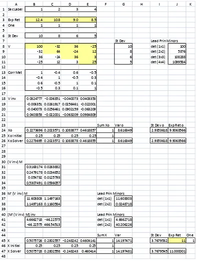
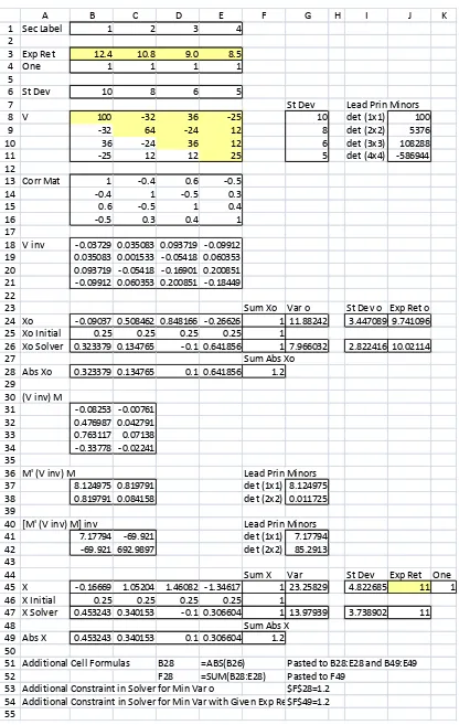
We now use two four-security cases to illustrate the positive de…niteness requirement. The only di¤erence between the two cases is in the covariance of returns between two speci…c securities. The covariance matrix in the …rst case is positive de…nite; the one in the second case is not. Figures 4a and 4b show part of an Excel worksheet for the …rst case. Here, the input parameters, consisting of
0 = 12:4 10:8 9:0 8:5 0
as measured in percentage terms, are provided in cellsB3:E3 and B8:E11, respectively.
The positive de…niteness of V is con…rmed by the positive sign of its four leading
principal minors, as shown in the cells J8:J11. As expected, all implied pairwise
cor-relations of security returns, as shown in cells B13:E16, are in the permissible range of
1to1:To …nd xo; o2;and o of the global minimum variance portfolio, we start with
V 1; which is shown in cells B18:E21. We …nd each element of the row vector x0
o by
dividing the corresponding 4-element column sum of the symmetricV 1 by the sum of
all its 16 elements; the result is displayed in cells B24:E24. The reciprocal of the sum
of all 16 elements of V 1;which is 2
o; is positive as expected; it is shown in cell G24.
Its square root, which is o; is shown in cell I24. With xo determined, o = x0o is
provided in cell J24.
We also use Solver to …nd xo; 2
o; and o: With the target cell G26 being for o2 =
x0
oV xo;we arbitrarily set equal weights of1=4for all four securities and paste these initial
values from cells B25:E25 to cells B26:E26. By changing the four portfolio weights in
cells B26:E26, Solver minimizes the target cell subject to the only constraint that the
sum of these portfolio weights, as captured by cell F26, be unity. As con…rmed by the
corresponding numbers in rows 24 and 26 of the Excel worksheet, theSolver results are
numerically the same as those based on equations (11)-(13).
To facilitate the computations for any predetermined expected return p based on
equations (9) and (10), we show in cells B31:C34,B37:C38, and B41:C42the computed
values of V 1M; M0V 1
M; and (M0V 1
M) 1
; respectively. As expected, the two
leading principal minors of M0V 1M;as shown in cells G37:G38, are positive. So are
the two principal minors of (M0V 1
A B C D E F G H I J K
7 St Dev Lead Prin Minors
8 V 100 -32 36 -25 10 det (1x1) 100
18 V inv 0.0324777 -0.006351 -0.040073 0.0403353 19 -0.006351 0.0261917 0.0256461 -0.022001 20 -0.040073 0.0256461 0.0902159 -0.063209 21 0.0403353 -0.022001 -0.063209 0.0984809 22
23 Sum Xo Var o St Dev o Exp Ret o
24 Xo 0.2273696 0.2023571 0.1083877 0.4618857 1 8.616349 2.9353618 9.9063566
25 Xo Initial 0.25 0.25 0.25 0.25 1
26 Xo Solver 0.2273695 0.2023572 0.1083878 0.4618855 1 8.616349 2.9353618 9.9063566 27
37 11.603803 1.1497163 det (1x1) 11.603803
38 1.1497163 0.1160584 det (2x2) 0.0248718
39
40 [M' (V inv) M] inv Lead Prin Minors
41 4.6662718 -46.22575 det (1x1) 4.6662718
42 -46.22575 466.54513 det (2x2) 40.206226
43
44 Sum X Var St Dev Exp Ret One
45 X 0.5075726 0.2802557 -0.248242 0.4604141 1 14.197471 3.7679532 11 1
46 X Initial 0.25 0.25 0.25 0.25 1
47 X Solver 0.5075728 0.2802558 -0.248243 0.460414 1 14.197481 3.7679545 11.000001 48
L M N O P Q R S T U 1
2 Cell Formulas B6 =SQRT(B8)
3 C6 =SQRT(C9)
13 B13 =B8/B$6/$G8 Pasted to B13:E16
14 B18:E21 {=MINVERSE(B8:E11)}
15
16 B24 =SUM(B18:B21)/SUM($B18:$E21) Pasted to B24:E24
17 F24 =SUM(B24:E24) Pasted to F24:F26
18 G24 =1/SUM(B18:E21)
19 I24 =IF(G24>0,SQRT(G24),"") Pasted to I26
20 J24 {=MMULT(B24:E24,TRANSPOSE(B$3:E$3))} Pasted to J26
21 G26 {=MMULT(B26:E26,MMULT(B8:E11,TRANSPOSE(B26:E26)))}
33 F45 =SUM(B45:E45) Pasted to F45:F47
34 G45 {=MMULT(B45:E45,MMULT(B$8:E$11,TRANSPOSE(B45:E45)))} Pasted to G47
35 I45 =IF(G45>0,SQRT(G45),"") Pasted to I47
36 J47 {=MMULT(B47:E47,TRANSPOSE(B3:E3))}
37 38
39 Solver for Min Var o Min $G$26
40 Changing Cells $B$26:$E$26
41 Constraint $F$26=1
42 43
44 Solver for Min Var with Given Exp Ret Min $G$47
45 Changing Cells $B$47:$E$47
46 Constraints $F$47=1
47 $J$47=$J$45
48
portfolio weight vector, x; and the corresponding variance and standard deviation of
portfolio returns, 2
p and p;for p = 11as an example, are shown in cellsB45:E45,G45,
and I45, respectively.
The above numerical results are also con…rmed by using Solver. The approach is
similar to that in the computations for the global minimum variance portfolio. The only
di¤erence is the additional constraint that the portfolio’s expected return,x0 ;as shown
in cellJ47, be equal to its predetermined value in cellJ45, which is11:Except for some
minor rounding errors, theSolver results, as shown in the corresponding cells in row 47,
are identical to the results based on equations (9) and (10).
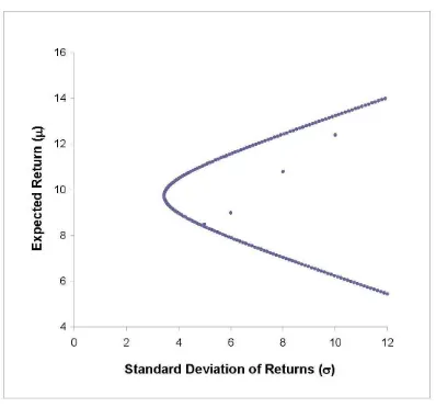
By repeating the computations based on these two equations for di¤erent values of
p;we are able to provide corresponding values of p and p for a graph on the( ; )
-plane. The graph, as shown in Figure 5, is generated by using Excel’s graphic feature
Charts, X Y (Scatter). The individual points of ( i; i);for i= 1;2;3;and 4;are also
shown. As expected, the graph is a branch of a hyperbola with a horizontal transverse axis. The upward-sloping part of the graph, starting from the global minimum variance portfolio, is the e¢cient frontier.
The input parameters for the Excel worksheet in Figure 6 di¤er from those in Figure
4a only in the covariance of returns between securities3 and 4;we have 34= 43= 12
instead of3:All implied correlations of returns, as shown in cellsB13:E16, are still in the
permissible range of 1 to1: Now, let us …rst consider the results in Figure 6 that are
based on equations (9)-(13). Speci…cally, the computed value of 2
o based on equation
(13) is positive, as shown in cellG24. The2 2matrix(M0V 1M) 1 has two positive
leading principal minors, as shown in cells G41:G42. The two portfolio variances as
shown in cells G24 and G45 are positive. Further, as shown in Figure 7, the graph on
the ( ; )-plane for di¤erent values of p and p is still a hyperbola with a horizontal
transverse axis. At …rst glance, as the graph has captured all the characteristics of minimum variance portfolios, equations (10)-(13) seem to have performed their intended tasks.
However, a closer inspection of Figure 6 reveals two problems. First, as shown in cell J11, the fourth leading principal minor — which is the determinant of the covariance matrix itself — is negative. Second, the inverse of the covariance matrix, as shown
in cells B18:E21, has three negative diagonal elements. Both are indications that the
covariance matrix is not positive de…nite. To show that the graph in Figure 7 does
not correspond to minimum variance portfolios, we …rst repeat the sameSolver runs in
Figure 4a with initially equal portfolio weights and with the default setting of Solver
options. The two portfolio variances as shown in cells G26 and G47, intended for 2
o
and 2
p; are 9:3 10
15
and 4:8 1015
; respectively. These results suggest that the
true value in each case is minus in…nity. Regardless of their true values, what is clear is that, with the covariance matrix not being positive de…nite, equations (10)-(13) do not correspond to any minimum variance portfolios.
As portfolio weights with extremely large magnitudes are unrealistic, we now restrict
such magnitudes in the Solver runs in order to illustrate that, if the covariance matrix
A B C D E F G H I J K
7 St Dev Lead Prin Minors
8 V 100 -32 36 -25 10 det (1x1) 100
18 V inv -0.03729 0.035083 0.093719 -0.09912 19 0.035083 0.001533 -0.05418 0.060353 20 0.093719 -0.05418 -0.16901 0.200851 21 -0.09912 0.060353 0.200851 -0.18449 22
23 Sum Xo Var o St Dev o Exp Ret o 24 Xo -0.09037 0.508462 0.848166 -0.26626 1 11.88242 3.447089 9.741096 25 Xo Initial 0.25 0.25 0.25 0.25 1
26 Xo Solver 0.323379 0.134765 -0.1 0.641856 1 7.966032 2.822416 10.02114
27 Sum Abs Xo
28 Abs Xo 0.323379 0.134765 0.1 0.641856 1.2 29 37 8.124975 0.819791 det (1x1) 8.124975 38 0.819791 0.084158 det (2x2) 0.011725 39
40 [M' (V inv) M] inv Lead Prin Minors 41 7.17794 -69.921 det (1x1) 7.17794 42 -69.921 692.9897 det (2x2) 85.2913 43
44 Sum X Var St Dev Exp Ret One
45 X -0.16669 1.05204 1.46082 -1.34617 1 23.25829 4.822685 11 1 46 X Initial 0.25 0.25 0.25 0.25 1
47 X Solver 0.453243 0.340153 -0.1 0.306604 1 13.97939 3.738902 11
48 Sum Abs X
49 Abs X 0.453243 0.340153 0.1 0.306604 1.2 50
variances lower than those based on equations (10)-(13). For the illustration, we
arbi-trarily restrict the sum of the absolute values of the four portfolio weights to be 1:2:
Thus, there is an additional constraint in eachSolver run. TheSolver results as shown
in row 26 of the Excel worksheet in Figure 6 indicate that a di¤erent set of portfolio weights can lead to a much lower variance of returns than that according to equation (13). Likewise, as shown in row 47, a di¤erent portfolio has a much lower variance of
returns than that according to equation (10) for p = 11:Thus, it is clear that, unless the
covariance matrix is positive de…nite, the portfolio results based on equations (10)-(13) do not correspond to minimum variance portfolios.
7
Concluding remarks
In …nance courses that are part of the core curriculum of business education, portfolio concepts are typically conveyed in terms of the correlations of security returns. For a given set of risky securities for portfolio investments, it is obvious that all pairwise
correlations of security returns must be in the permissible range of 1 to 1: However,
standard investment textbooks are silent on whether there are any other requirements on the variances and covariances of security returns.
In contrast, it is well-known in the academic …nance literature that, when the vari-ances and covarivari-ances are arranged as elements of a symmetric matrix, called the co-variance matrix of security returns, such a matrix must satisfy a speci…c requirement in order to be meaningful. This study has considered the requirement from a pedagogic perspective. In the language of matrix algebra, the requirement is that the covariance matrix be positive de…nite. In the context of portfolio investments under the assumption of frictionless short sales, a positive de…nite covariance matrix ensures that the variance of portfolio returns be always positive, regardless of how investment funds are allocated among the securities considered.
The positive de…niteness requirement is crucial because its violation will prevent portfolio selection models from performing their intended tasks. With the aid of Excel tools, this study has revealed some consequences of its violation. Of special relevance is that its violation does not preclude the attainment of a hyperbola — which is intended to capture the achievable risk-return trade-o¤ from portfolio investments — with a
hor-izontal transverse axis on the plane of standard deviation of returns ( )and expected
return ( ); where is the horizontal axis. As students are taught that the e¢cient
frontier, starting from the global minimum variance portfolio, is a concave curve on the
( ; )-plane, violation of the positive de…niteness requirement may appear to be
incon-sequential at …rst glance. Nevertheless, it is such a situation that can cause serious confusion for students.
This study has shown that, if the positive de…niteness requirement is violated, the analytical results will not correspond to constrained minimization of the variance of portfolio returns as intended. That is, some other allocations of investment funds satis-fying the same constraints can lead to lower variances of portfolio returns. If so, Excel
for providing numerical illustrations. This study has provided various Solver illustra-tions, thus helping students understand better the positive de…niteness requirement and implications for its violations.
BesidesSolver, Excel functions for basic matrix operations are also useful for teaching
mean-variance portfolio analysis. They include matrix transposition, multiplication, and inversion, as well as …nding the determinant of a matrix. To allow the positive de…niteness requirement and implications of its violations to be covered e¤ectively in the classroom, we as instructors must ensure that students are completely at ease with basic matrix operations. As matrix operations in Excel are easy to follow, students can focus on relevant analytical issues without being encumbered by the attendant computational chores. This study has illustrated with examples how various Excel features can be used for pedagogic purposes.
In order to make the analytical materials self-contained, this study has included several algebraic proofs that are set at levels accessible to business students with gen-eral analytical skills. The materials as presented in this study can be used in di¤erent ways, depending on the pedagogic approaches of the investment courses involved. For classes where an informal approach is intended for illustrating the positive de…niteness requirement, neither the basic portfolio selection model nor the various proofs involved are essential. For advanced investment classes, however, such proofs — in the form of either lecture materials or exercises for students — can facilitate a better understanding of the basic portfolio selection model by students.
Acknowledgement
The author wishes to thank the anonymous reviewers for helpful comments and sugges-tions.
References
[1] Cheung, C.S., Kwan, C.C.Y., and Miu, P.C. (2007). “Mean-Gini Portfolio Analysis:
A Pedagogic Illustration,”Spreadsheets in Education,2(2), Article 3.
[2] Gilbert, G.T. (1991). “Positive De…nite Matrices and Sylvester’s Criterion,”
Amer-ican Mathematical Monthly,98(1), 44–46.
[3] Jobson, J.D., and Korkie, B. (1989). “A Performance Interpretation of Multivariate
Tests of Asset Set Intersection, Spanning, and Mean-Variance E¢ciency,” Journal
of Financial and Quantitative Analysis,24(2), 185–204.
[4] Johnson, C.R. (1970). “Positive De…nite Matrices,” American Mathematical
Monthly,77(3), 259–264.
[5] Kwan, C.C.Y. (2006). “Some Further Analytical Properties of the Constant
Cor-relation Model for Portfolio Selection,” International Journal of Theoretical and
[6] Kwan, C.C.Y. (2007). “A Simple Spreadsheet-Based Exposition of the Markowitz
Critical Line Method for Portfolio Selection,” Spreadsheets in Education,2(3),
Ar-ticle 2.
[7] Kwan, C.C.Y. (2008). “Estimation Error in the Average Correlation of Security
Re-turns and Shrinkage Estimation of Covariance and Correlation Matrices,” Finance
Research Letters, 5, 236–244.
[8] Kwan, C.C.Y. (2009). “Estimation Error in the Correlation of Two Random
Vari-ables: A Spreadsheet-Based Exposition,” Spreadsheets in Education, 3(2), Article
2.
[9] Ledoit, I., and Wolf, M. (2004). “Honey, I Shrunk the Sample Covariance Matrix,”
Journal of Portfolio Management (Summer), 110–119.
[10] Martin, R.S., Peters, G., and Wilkinson, J.H. (1965). “Symmetric Decomposition
of a Positive De…nite Matrix,” Numerische Mathematik,7, 362–383.
[11] Merton, R.C. (1972). “An Analytic Derivation of the E¢cient Portfolio Frontier,”
Journal of Financial and Quantitative Analysis,7(4), 1851–1872.
[12] Roll, R. (1977). “A Critique of the Asset Pricing Theory’s Tests, Part I: On Past and
Potential Testability of the Theory,” Journal of Financial Economics,4, 129–176.
Appendix A
This appendix shows that the sample covariance matrix is always positive semide…nite.
The proof starts with de…ning Rit as the return of security i observed at time t; for
i = 1;2; : : : ; n and t = 1;2; : : : ; T; where T is the number of return observations. Let
be the sample covariance of returns between securitiesiandj; whereRi and Rj are the
corresponding sample mean returns, for i; j = 1;2; : : : ; n; including i= j: The sample
covariance matrixVb is ann nmatrix with each element (i; j) being bij:
To show thatVb is positive semide…nite, let
uit=
t;which is never negative. Withxand,
conse-quently,wbeing arbitrary, the positive semide…niteness of the sample covariance matrix
Notice that, if there are insu¢cient observations (withT < n) for the estimation of
the covariance matrix, we can writeVb =U U0 =ZZ0;whereZ= U 0 is ann n
matrix formed by appending then T matrixU with ann (n T) matrix0with all
zero elements. The determinant of Vb is zero, as it is the product of the determinants
of Z and Z0; both of which are zeros. Although Vb in this situation is not invertible,
it is still positive semide…nite. Whether the sample covariance matrix is invertible is irrelevant in the proof of its positive semide…niteness.
Notice also the following, regardless of whether there are su¢cient observations:
1. IfRi1 =Ri2= =RiT;securityiis risk-free. AsRi1 Ri; Ri2 Ri; : : : ; RiT Ri
are zeros, rowiof U has all zero elements. A vectorxwhere element iis its only
non-zero element will result inw being a vector of zeros.
2. For two risky securities i and j; ifRit=a+bRjt fort= 1;2; : : : ; T; wherea and
b are constants, the returns of the two securities are perfectly correlated. In such
a case, knowing one of Rit and Rjt will enable us to determine the remaining one
directly for any t: As Rit Ri = b(Rjt Rj); a vector x with its only non-zero
elements being 1 and b for elements i and j; respectively, will make w consist
only of zero elements.
3. IfRitas observed at anytcan be replicated exactly by the same linear combination
of some of the remaining returns amongR1t; R2t; : : : ; Rnt;in the form of
be made a vector of zeros as well. The reason is that, with
Rit Ri =
to ensure that w be a vector of zeros. Equation (A3) encompasses, as a special
case, the situation where security i is a portfolio of some other securities among
then securities; in such a case, we havea= 0 and Pik=11 bk+Pnk=i+1bk = 1:
Appendix B
For more elegant proofs of Sylvester’s criterion, see, for example, Johnson (1970) and Gilbert (1991). The proof below requires only matrix properties that are accessible to business students with general algebraic skills. Let us start with the de…nition of
determinant. The determinant of an n n matrix V;where each element (i; j) is ij;
i1; i2; : : : ; in:Thendi¤erent integers thati1; i2; : : : ; inrepresent can be any permutation
of 1;2; : : : ; n: If it takes an even number of inversions (interchanges), each involving an
adjacent pair of integers in the sequence, to rearrange these integers as 1;2; : : : ; n; the
sign factor for 1i1 2i2 nin is(+1):If it takes an odd number of inversions, the sign
factor is( 1)instead.12 Here, we label the determinant of V asdetV:
Suppose that we wish to …nd a parameter and a correspondingn-element non-zero
column vectorxsatisfying the equationV x= x:In the language of matrix algebra, is
an eigenvalue and the correspondingxis an eigenvector. As the equation can be written
as(V I)x =0; where I is an n n identity matrix and 0 is an n-element column
vector of zeros, the existence of a solution requires that the determinant of V I be
zero. The equation det(V I) = 0 is called the characteristic equation. The idea
is that, if det(V I) 6= 0; the matrix V I is invertible and the resulting vector
x= (V I) 1
0 will inevitably be a vector of zeros. The characteristic equation being
a polynomial equation of degreen; there arenpotential values of ;which need not be
all distinct.
As the product of the n diagonal elements of V I; which is ( 11 )( 22
) ( nn );provides the highest power of in the expression ofdet(V I);we can
write the expression as a polynomial function P( ): The coe¢cient of n; the highest
power term in P( ); is ( 1)n: The existence of n eigenvalues of ; labeled as
i; for
i= 1;2; : : : ; n;implies that
P( ) = ( 1)n(
1)( 2) ( n) = 0: (B1)
The value of this polynomial function at = 0;
P(0) = ( 1)n( 1)( 2) ( n) = 1 2 n; (B2)
is alsodetV:Thus, the determinant of ann nmatrix is the product of itsneigenvalues.
A crucial matrix property as required for proving Sylvester’s criterion is that all eigenvalues of a real symmetric matrix are real. To prove this property, let us assume
that, contrary to the assertion, each is of the forma+bp 1;where bothaandbare real.
The complex conjugate ofa+bp 1isa bp 1;by changing the sign of the imaginary
part of the expression. Notice that (p 1)2
= 1 and that (a+bp 1)(c+dp 1) =
(a+bp 1) (c+dp 1);wherec anddare also real and each algebraic expression with
a bar above it represents its complex conjugate. Thus, for any speci…c eigenvalue ;
we can write the equation V x = x as V x = x; by taking the complex conjugates
of both sides of the equation. Suppose that the corresponding eigenvector x is a
non-zero vector, with each element written generally in the form of a+bp 1: We can also
write x0x= (x0x)0 =x0x >0;because the three matrix products here, each being the
sum ofn positive terms of the form a2
+b2
per term, will all result in the same scalar.
1 2For example, in the case ofn= 3;the sequence3;2;1requires three inversions to reach1;2;3: The
Combiningx0V x= x0xand x0V x= x0xleads to
x0V x x0V x= ( )x0x: (B3)
As V is symmetric, the left hand side of equation (B3) is zero. Thus, we must have
= ; that is, each eigenvalue ofV must be real. Notice that, with all elements of the
matrixV I being real for each speci…c eigenvalue ;we can choose the corresponding
eigenvectorxthat satis…es the equation (V I)x=0 to be a real vector.
To prove the part of Sylvester’s criterion that, if V is positive de…nite, its leading
principal minors are all positive, we …rst draw on the result thatx0V x= x0xis positive
for any real eigenvector x associated with each speci…c eigenvalue : With x0x being
positive, it follows that the corresponding is positive. As the determinant of a matrix
is the product of its eigenvalues according to equation (B2), detV; which is the n-th
leading principal minor of V; is positive as well. Further, the n n matrix V being
positive de…nite, the scalarx0V xfor anyn-element non-zero column vectorxis positive.
Form= 1;2; : : : ; n 1;if the lastn m elements ofxare set to be zeros, the condition
of x0V x > 0 is equivalent to x0
mVmxm > 0; where Vm is the m-th leading principal
submatrix of V and xm is an arbitrary m-element non-zero column vector. With each
Vm being positive de…nite, it follows that the correspondingdetVm is positive.
To prove, by induction, the part of Sylvester’s criterion that, if all leading principal
minors ofV are positive,V is positive de…nite, we start with the …rst leading principal
submatrix of V; labeled as V1; which consists of a single element, 11: Obviously, if
11>0;any single-element non-zero vectorx1 will give usx01V1x1>0;con…rming that
V1 is positive de…nite. Now, suppose that, by inductive hypothesis,detV1;detV2; : : : ;
detVn are all positive and Vn is positive de…nite. The task now is to show that, if
detVn+1 is positive, Vn+1 is positive de…nite.
Lettingv = 1;n+1 2;n+1 n;n+1 0;ann-element column vector consisting
of the …rstnelements of the last column ofVn+1;we can writeVn+1=Q0BQ;a product
of three(n+1) (n+1)matrices. Here,Bis constructed by augmenting then nmatrix
Vn with both a rown+ 1and a column n+ 1of zeros, except for element(n+ 1; n+ 1);
which is an unspeci…ed parameter g: The matrix Q is constructed by substituting the
…rst n elements of the last column of an (n+ 1) (n+ 1) identity matrix with n
elements of the column vectorVn1v:As it will soon be clear, althoughg can be solved
in terms of the elements ofVn+1;there is no need to do so for the purpose here. We can
where Qxn+1 is an (n+ 1)-element column vector. Let us label the vector consisting
of the …rst n elements of Qxn+1 as yn and the last element as h: Equation (B4) now
becomes
x0n+1Vn+1xn+1=y0nVnyn+gh
2