Directory UMM :Data Elmu:jurnal:J-a:Journal of Economics and Business:Vol51.Issue2.Mar1999:

Anticipated, Unanticipated Expansionary,

and Unanticipated Contractionary

Monetary Policy

Joonsuk Chu and Ronald A. Ratti

It has been found that distinctions among positive innovations, negative innovations, and

anticipated monetary policy change are relevant for explaining movement in real output.

An asymmetry in the effects of anticipated expansionary and anticipated contractionary

monetary policy on output also was found to be statistically significant, and the null

hypothesis of no asymmetry in stimulative/contractionary policy was rejected. There is

evidence that unanticipated stimulative, unanticipated contractionary, anticipated

stimu-lative, and anticipated contractionary monetary policy each have statistically significant

effects on output. Recognition of these asymmetries was found to make the finding of

non-neutrality more likely.

© 1999 Elsevier Science Inc.

Keywords:

Expansionary; Contractionary; Monetary policy

JEL classification:

E52, E58

I. Introduction

The policy ineffectiveness proposition advanced by Lucas (1973) and Sargent and

Wallace (1975) conjectures that anticipated nominal changes have no effect on real output.

The hypothesis that differentiation between anticipated and unanticipated change in

nominal variables is important for explaining movement in real output was tested by Barro

(1977), who found support for the neutrality hypothesis. In contrast, Mishkin (1982) found

that when lag length was increased in the nominal variables, the neutrality hypothesis was

Youngsan University of International Affairs, Yangsan, Korea (JC); Department of Economics, University of Missouri-Columbia, Columbia, Missouri (RAR).

Address correspondence to: Dr. R. A. Ratti, University of Missouri-Columbia, Department of Economics, 118 Professional Building, Columbia, MO 65211.

rejected. In a further extension, Frydman and Rappoport (1987) presented evidence

casting doubt on the relevance of the distinction itself between anticipated and

unantic-ipated nominal change in explaining real output. Work by De Long and Summers (1988)

and Cover (1992) has drawn attention to a different asymmetry and concluded that

negative-money shocks have a greater effect on output than positive-money shocks.

1

Macklem et al. (1996) found evidence for Canada that asymmetric effects on output exist

in anticipated policy.

2

This paper examines the relevance of distinctions among anticipated monetary policy

change, unanticipated positive-money change, and unanticipated negative-money change

in explaining movement in real output. The role of a possible asymmetry in policy actions,

e.g., stimulative versus contractionary policy, is also considered.

3

Growth in M1 will be

one of the measures of monetary policy. The spread between the commercial paper rate

and the Treasury bill rate will be another. Work by Friedman and Kuttner (1992) indicates

that spread contains highly significant information about movement in real output.

Kashyap et al. (1993) viewed spread as a proxy for the stance of monetary policy. A tight

monetary policy causes firms to compete for funds, leading to an increase in the issuance

of commercial paper. Hence, the commercial paper rate rises more than the Treasury bill

rate when money is tight.

4

The change in the federal funds rate will also be used as a measure of monetary policy.

This will allow the issue of possible asymmetry in the effects of anticipated policy to be

tested.

5

Bernanke and Blinder (1992) have argued that innovations in the federal funds

1_{Cover (1992, p. 1261) went so far as to state that “positive-money shocks have no effect on output, whereas} negative-money shocks cause output to decline.” Cover noted that this outcome is consistent with either a rigidly vertical aggregate supply curve and sticky prices in the face of unexpected changes in demand, or with a situation in which wages are sticky downwards but flexible upwards and a vertical aggregate supply curve at the point of full employment. A zero effect of positive money shocks is, of course, not predicted by either the new classical model with rational expectations, in which prices are flexible, or the nonclassical rational expectations model with contracts. Recent work by Lucas (1990), Christiano (1991), and Fuerst (1992) within a cash-in-advance real business-cycle framework, provides some motivation for assuming an asymmetry in the effect of positive and negative money shocks, but not a basis for concluding that positive shocks are unimportant.

2_{A number of papers have addressed ways in which there may be asymmetric effects of policy on the real} economy. This includes work by Bernanke and Gertler (1989), Caplin and Leahy (1991), and Ball and Mankiw (1994). Empirical evidence of asymmetric effects of monetary policy has been reported by Morgan (1993), Huh (1994), Thoma (1994), Ammer and Brunner (1995), and Garcia and Schaller (1995). Macklem et al. (1996) provide an excellent survey of work on asymmetric effects of monetary policy.

3_{In this paper, monetary policy innovations are formed by using a method used by Mishkin (1982), Cover} (1992), and Macklem et al. (1996). This involves a forecast equation for the monetary policy indicator. Residuals from this equation are then used as innovations to be used in an output equation. This method of construction contrasts with that used to identify policy shocks in a large literature using structural vector autoregression (VAR) models [see, for example Sims (1980, 1992); Bernanke (1986); Bernanke and Blinder (1992)]. Cochrane (1995) argued that the VAR technique implicitly assumes that only unanticipated shocks matter. Bernanke and Mihov (1995) and Cochrane (1995) maintained that it is important to allow for the possible effect of anticipated money on output. In addition, Macklem et al. (1996) stressed that when asymmetric effects are being considered, scarcity of degrees of freedom becomes even more of a problem with the VAR approach.

4_{Friedman and Kuttner (1992) held that the gap between the Commercial Paper rate and the Treasury bill} rate better captures information about occurrences in financial markets relevant for the determination of output than movements in an interest rate or fluctuations in money. In another paper, Friedman and Kuttner (1993) point out that monetary policy is only one of several factors that can account for movement in spread and its relationship to output. Kashyap et al. (1993) have shown that monetary policy influences a firm’s mix of external financing and that this implies that a loan supply channel of monetary policy exists.

rate are a good measure of changes in monetary policy and are informative about future

movements in real activity.

6

It was found in our study that distinctions between positive innovations, negative

innovations, and anticipated monetary policy change are relevant for explaining

move-ment in real output. There is evidence that unanticipated expansionary monetary policy is

just as likely to have a statistically significant effect on output as is unanticipated

contractionary monetary policy.

7

These results appear to be robust across different

measures of monetary policy, different specifications of the monetary policy and output

equations, and over different sample periods.

For monetary policy measured by change in the federal funds rate, an asymmetry in the

effects of anticipated expansionary and anticipated contractionary monetary policy on

output was found. The null hypothesis of no asymmetry in stimulative/contractionary

policy was rejected. Anticipated expansionary monetary policy and anticipated

contrac-tionary policy were each found to have statistically significant effects on output. A major

finding of the study is that allowing asymmetries in anticipated and unanticipated

monetary policy between stimulative and contractionary components makes the finding of

neutrality of money less likely.

In Section II, the model and the hypotheses to be considered are presented. Empirical

results for growth in money and for spread are presented in Sections III and IV,

respectively. The issue of asymmetry in stimulative/contractionary policy is taken up in

Section V, when the change in the federal funds rate is used as the measure of monetary

policy. Section VI is the conclusion.

II. The Model and Hypotheses

The procedure adopted in this paper involves nonlinear joint estimation of a money policy

indicator equation—from which monetary policy innovations will be constructed—and a

real output growth equation. The setup of the relationship between money and output

follows that in Barro (1977) and Mishkin (1982).

8

The monetary policy indicator process

is characterized by:

MPI

t

5

Z

t21

g 1

u

t

,

(1)

where

t

5

2, . . . ,

T

. In equation (1), the monetary policy indicator,

MPI

t

, can be

represented by the growth in M1, spread, the change in the federal funds rate, or some

other measure of the stance of monetary policy.

Z

t21

is a vector of variables used to

forecast

MPI

t

available at time

t

2

1, and

g

is a vector of coefficients.

u

t

is an error term

assumed to be serially uncorrelated and independent of

Z

t21

.

The output equation is initially given in difference stationary form by:

6_{Bernanke and Blinder (1992) argued that the forecasting performance of the federal funds rate is based on} sensitivity to changes in bank reserves. They also felt that a credit channel is at work in the monetary transmission mechanism.

GY

t

5

a

0

1

O

In equation (2),

GY

t

is growth in real gross domestic product;

W

t

is a vector of variables

influential in determining real growth;

u

is a vector of coefficients, and

e

_t

is an error term.

9

The

b

_iu1

,

b

_iu2

,

b

_ie

,

i

5

0, 1, . . .

n

, are the effects of positive innovations (

MPI

t2i

) monetary policy on real growth,

respec-tively. In a later section of the paper, when the change in the federal funds rate is

considered as the monetary policy indicator, anticipated monetary change will also be

separated into positive and negative components. This will allow the possible role of

asymmetry in stimulative/contractionary policy to be considered.

The residuals from equation (1),

uˆ

t

, form the basis for measures of monetary policy

indicator shocks and anticipated monetary policy used in equation (2). A positive

mon-etary policy shock is defined as

MPI

t

u1

₅

uˆ

t

if

uˆ

t

is positive; otherwise, it equals zero. A

negative monetary policy shock is defined as

MPI

t u2

₅

uˆ

t

if

uˆ

t

is negative; otherwise it

equals zero. Anticipated monetary policy for time

t

is defined as

MPI

t e

₅

Z

t21

g

ˆ

. For MPI

given by growth in M1, Cover (1992) jointly estimated equations (1) and (2), and tested

the null hypothesis that the positive-negative innovation distinction is irrelevant for

explaining output (henceforth, PNDI) by testing

b

_iu1

5

b

_iu2

,

i

5

0, 1, . . .

n

. Cover found

that PNDI was rejected, and that the null hypothesis

b

_iu1

5

0,

i

5

0, 1 . . .

n

, could not

be rejected.

10

The hypotheses to be tested are basically checks for asymmetries of one type or

another. Frydman and Rappoport (1987) tested the null hypothesis that the

anticipated-unanticipated distinction is irrelevant (AUDI) for explaining output by implicit imposition

of the restriction that

b

_iu1

5

b

_iu2

(

5

k

_iu

),

i

5

0, 1, . . .

n

. The difference stationary form of

their output equation is given by:

GY

t

5

a

0

1

O

They reported results for

n

$

7 for M1 over the period 1954:I–1976:IV which suggested

AUDI could not be rejected.

This paper examines the null hypothesis that distinctions among anticipated monetary

policy, unanticipated positive policy shocks, and unanticipated negative policy shocks are

irrelevant for explaining output (

SYMMETRY

).

SYMMETRY

will be tested by setting up

the null hypothesis of

b

_iu1

5

b

_iu2

5

b

_ie

,

i

5

0, 1, . . .

n

.

11

_{It is argued in this paper that}

a distinction between anticipated and unanticipated monetary policy shocks might be

9_{Analysis of the time series properties ofGY}

tindicated a stationary process. With the presence of money

shock terms in equation (2), tests indicated that the error term does not show first-order or higher-order serial correlation.

10_{The Cover (1992) conclusion that expansionary monetary has statistically insignificant effects on output} was formed given imposition of the constraint thatbi

e_{50,i50, 1, . . .n.}

11_{Note that if SYMMETRY cannot be rejected, equation (2) reduces down to an equation in which} expectations about monetary policy do not affect output, asMPIt2i

rejected by failure to account for a possible asymmetry between positive and negative

monetary policy surprises. It is also contended that if such an asymmetry exists in effects

on output, taking account of this distinction will affect findings on neutrality.

The underlying reason for these results can be seen intuitively by supposing that the

true output equation is given by equation (2). In this case, the error term in equation (3)

is defined as:

Equation (4) demonstrates that in equation (3),

h

_t

is not orthogonal to the

MPI

t2i u

estimators of the parameters in equation (3) and inconsistent test statistics on hypotheses

concerning these parameters.

12

The estimation procedure is as follows. Equations (1) and (2) are estimated by OLS. In

equation (2),

MPI

t2i

u1

_and

MPI

t2i u2

₍

i

5

0, 1, . . .

n

) have been given by the residuals from

equation (1). In this second stage,

n

is determined by the Akaike (1973) Information

Criterion (AIC). The OLS residuals of both equations are used to construct the

variance-covariance matrix for the system, and equations (1) and (2) are re-estimated jointly by

nonlinear generalized least-squares, treating the estimated variance-covariance matrix as

given. It is assumed that the residuals in the monetary policy equation and in the output

equation are uncorrelated. A new variance-covariance matrix is re-estimated with each

new set of coefficient estimates until the change in this estimated matrix is infinitesimal.

13

III. Empirical Results for M1

To separate monetary policy into anticipated and unanticipated positive and negative

components, growth in M1 (

GM

) is regressed on lagged values of itself, lagged values of

growth in the monetary base (

GB

), lagged values of the unemployment rate (

UR

), lagged

growth rates of GDP (

GY

), lagged changes in the T-bill rate (

DTBR

), and lags of the

federal government surplus (

FEBS

).

14

_{This specification is similar to that in Mishkin}

(1982), Frydman and Rappoport (1987), and Cover (1992). The growth rate in output is

regressed on lag distributions of

MG

e

,

MG

u1

, and

MG

u2

, and lags of changes in the

Treasury-bill rate and growth in output.

15

_{Results of joint estimation of money and output}

12_{It should also be noted that inconsistent estimators might be obtained if an asymmetry exists in anticipated} policy. However, for measures of monetary policy given by growth in M1 and spread, it is not possible with the method outlined above to identify stimulative and contractionary components of anticipated policy. This issue is considered when change in the federal funds rate is used as measure of monetary policy.

13_{This procedure iterated until the relative change in the value of the function was less than 0.000001. The} BHHH algorithm was used for optimization. The resulting estimates are approximately maximum-likelihood estimates [Mishkin (1982, p. 26)]. The coefficient estimates obtained from joint estimation are more efficient because of cross-equation restrictions.

14_{Data are from CITIBASE, except for M1 prior to 1959:I. As in Cover (1992), M1 during the third month} of the quarter was used as the money supply. Prior to 1959:I, data on M1 obtained from Friedman and Schwartz (1970) was multiplied by 0.990302 (the ratio of the M1 series in CITIBASE to the M1 series in Friedman and Schwartz for the period 1959:I–1960:IV).

equations for

n

5

4 appear in Tables 1 and 2 for the period 1951:I–1979:III, and in Tables

1 and 3 for the period 1951:I–1992:II.

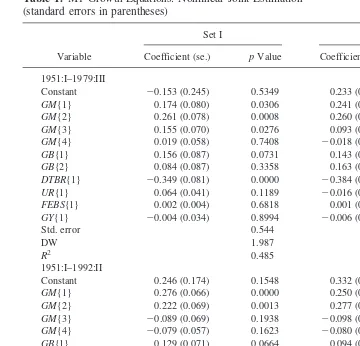
16

Money equations are reported in Table 1 and

output equations in Tables 2 and 3. In these tables, Set I corresponds to equations (1) and

(2), and Set II corresponds to equations (1) and (3).

results on an asymmetry between positive and negative policy shocks. Note that lagged changes in the Treasury-bill rate were found to be statistically significant in the output equations.

16_{Results for the period ending in 1979:III are reported, as during October 1979, Fed operating procedures} changed and results could be more easily compared with those obtained by Barro and Rush (1980), Mishkin (1982), and Frydman and Rappoport (1987). Results are also reported for the period ending in 1992:II. This provides an update and also facilitates comparison with the work of Cover (1992), whose sample period ended in 1987:IV.n54 was chosen by AIC applied to the initial OLS estimate of the output equation. Results for higher values ofnwill be reported.

Table 1. M1 Growth Equations: Nonlinear Joint Estimation (standard errors in parentheses)

Variable

Set I Set II

Coefficient (se.) pValue Coefficient (se.) pValue

1951:I–1979:III

Constant 20.153 (0.245) 0.5349 0.233 (0.180) 0.1933

GM{1} 0.174 (0.080) 0.0306 0.241 (0.085) 0.0044

GM{2} 0.261 (0.078) 0.0008 0.260 (0.089) 0.0035

GM{3} 0.155 (0.070) 0.0276 0.093 (0.077) 0.2272

GM{4} 0.019 (0.058) 0.7408 20.018 (0.066) 0.7793

GB{1} 0.156 (0.087) 0.0731 0.143 (0.086) 0.0957

GB{2} 0.084 (0.087) 0.3358 0.163 (0.095) 0.0866

DTBR{1} 20.349 (0.081) 0.0000 20.384 (0.091) 0.0000

UR{1} 0.064 (0.041) 0.1189 20.016 (0.028) 0.5590

FEBS{1} 0.002 (0.004) 0.6818 0.001 (0.002) 0.5836

GY{1} 20.004 (0.034) 0.8994 20.006 (0.039) 0.8670

Std. error 0.544 0.549

DW 1.987 2.057

R2 _{0.485 0.475}

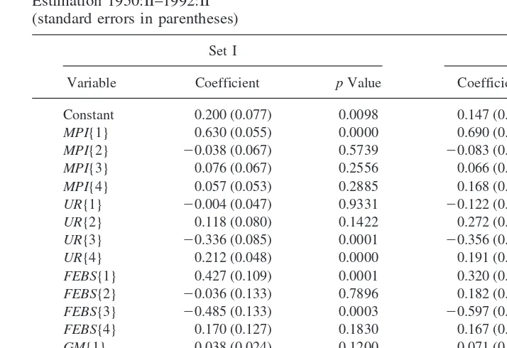
1951:I–1992:II

Constant 0.246 (0.174) 0.1548 0.332 (0.173) 0.0551

GM{1} 0.276 (0.066) 0.0000 0.250 (0.070) 0.0003

GM{2} 0.222 (0.069) 0.0013 0.277 (0.075) 0.0002

GM{3} 20.089 (0.069) 0.1938 20.098 (0.071) 0.1681

GM{4} 20.079 (0.057) 0.1623 20.080 (0.058) 0.1682

GB{1} 0.129 (0.071) 0.0664 0.094 (0.061) 0.1232

GB{2} 0.114 (0.073) 0.1149 0.093 (0.062) 0.1295

DTBR{1} 20.399 (0.048) 0.0000 20.371 (0.050) 0.0000

UR{1} 0.030 (0.029) 0.3120 0.015 (0.029) 0.5819

FEBS{1} 20.002 (0.001) 0.0816 20.002 (0.001) 0.0079

GY{1} 0.025 (0.043) 0.5495 0.031 (0.044) 0.4685

Std. error 0.713 0.713

DW 2.006 1.923

R2 _{0.509 0.509}

From the Set I results in Tables 1, 2, and 3, it can be seen that the null hypothesis—that

distinctions among the effects of

MG

e

,

MG

u1

, and

MG

u2

on growth in output are

irrelevant (

SYMMETRY

)—is rejected at the 0.05 level for both time periods. From the Set

II results, it is also apparent that AUDI is also rejected. These results are summarized in

the first column of the upper part of Table 4 which brings together a number of results as

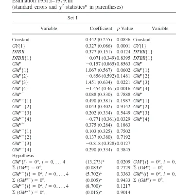
Table 2. Output Equations with Growth in M1 as Monetary Policy Indicator: Nonlinear Joint Estimation 1951:I–1979:III

(standard errors andx2_{statistics* in parentheses)}

Set I Set II

Variable Coefficient pValue Variable Coefficient pValue

Constant 0.442 (0.255) 0.0836 Constant 0.859 (0.404) 0.0334

GY{1} 0.327 (0.086) 0.0001 GY{1} 0.256 (0.134) 0.0549

DTBR 0.377 (0.151) 0.0124 DTBR{1} 0.280 (0.159) 0.0777

DTBR{1} 20.071 (0.349) 0.8395 DTBR{1} 20.883 (0.607) 0.1455

GMe _{20.157 (0.865) 0.8563 GM}e _{22.195 (1.395) 0.1157}

GM3_{{1} 1.067 (0.567) 0.0602 GM}e_{{1} 1.486 (0.656) 0.0234}

GMe_{{2} 20.856 (0.592) 0.1481 GM}e_{{2} 0.094 (0.724) 0.8965}

GMe_{{3} 1.451 (0.634) 0.0221 GM}e_{{3} 1.513 (0.591) 0.0104}

GMe_{{4} 21.454 (0.461) 0.0016 GM}e_{{4} 21.080 (0.419) 0.0099}

GMu2 _{0.088 (0.330) 0.7888 GM}u _{0.347 (0.153) 0.0235}

GMu2_{{1} 0.490 (0.381) 0.1987 GM}u_{{1} 0.939 (0.477) 0.0488}

(5)-test of the null hypothesis that the coefficients onGMe

(GMu1

,GMu2

, orGMu

) terms are jointly zero.

b_x2

(1)-test of the null hypothesis that the sum of the coefficients on theGMe

(GMu1

(10)-test of joint pairwise equality and of joint triple-wise equality, respectively, of coefficients on variables indicated.

d_x2

(1)-test andx2

(2)-test of pairwise equality and of triple-wise equality, respectively, of sums of coefficients on variables indicated.

GMe

{i},GMu2

{i}, andGMu1

lag distributions of the nominal variables are increased. For example, for

n

5

8 and

greater, the result noted by Frydman and Rappoport (1987), of the

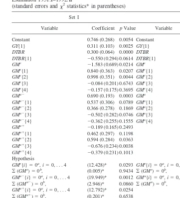
anticipated-Table 3. Output Equations with Growth in M1 as Monetary Policy Indicator: Nonlinear Joint Estimation 1951:I–1992:II

(standard errors andx2_{statistics* in parentheses)}

Set I Set II

Variable Coefficient pValue Variable Coefficient pValue

Constant 0.746 (0.268) 0.0054 Constant 0.661 (0.264) 0.0122

GY{1} 0.311 (0.103) 0.0025 GY{1} 0.343 (0.121) 0.0045

DTBR 0.300 (0.064) 0.0000 DTBR 0.270 (0.065) 0.0000

DTBR{1} 20.550 (0.294) 0.0614 DTBR{1} 20.749 (0.292) 0.0103

GMe _{21.583 (0.689) 0.0214 GM}e _{22.126 (0.740) 0.0040}

GMe_{{1} 0.840 (0.363) 0.0207 GM}e_{{1} 1.077 (0.406) 0.0079}

GMe_{{2} 0.998 (0.351) 0.0044 GM}e_{{2} 1.277 (0.423) 0.0025}

GMe_{{3} 20.084 (0.201) 0.6743 GM}e_{{3} 20.204 (0.234) 0.3834}

GMe_{{4} 20.157 (0.175) 0.3695 GM}e_{{4} 20.151 (0.206) 0.4607}

GMu2 _{0.690 (0.193) 0.0003 GM}u _{0.219 (0.090) 0.0156}

GMu2_{{1} 0.537 (0.306) 0.0789 GM}u_{{1} 0.558 (0.283) 0.0485}

(5)-test of the null hypothesis that the coefficients onGMe

(GMu1

,GMu2

, orGMu

) terms are jointly zero.

b_x2

(1)-test of the null hypothesis that the sum of the coefficients on theGMe

(GMu1

(10)-test of joint pairwise equality and of joint triple-wise equality, respectively, of coefficients on variables indicated.

d_x2

(1)-test andx2

(2)-test of pairwise equality and of triple-wise equality, respectively, of sums of coefficients on variables indicated.

GMe

{i},GMu2

{i}, andGMu1

unanticipated distinction being irrelevant for the period 1954:I–1976:IV, comes into play

(on the first line of Table 4).

17

Note however that these results on the rejection of AUDI contrast sharply with those

obtained at longer lags when distinctions among positive shocks, negative shocks, and

anticipated money growth are simultaneously allowed. The null hypothesis that

distinc-tions among the three types of monetary change are irrelevant is rejected at the 0.01 level

for

n

$

8 for the period ending in 1979:III. In comparison to the conclusion of Frydman

and Rappoport, it appears that distinctions between anticipated and unanticipated changes

in nominal values do matter for explaining movement in output, at least when a distinction

is allowed between the impact of positive and negative shocks. This outcome is relatively

stable for both sample periods and over various lag lengths.

As reported in Table 5, at longer lags for both sample periods, the null hypotheses that

neither positive money nor negative money surprises have an effect on output is rejected

at the 0.05 level. Thus positive money surprises matter (as do negative money surprises).

This result seems to differ from that reported by Cover (1992), to the effect that positive

17_{Frydman and Rappoport (1987) reported results for a period ending in 1976:IV and forn$7. They stated} that results with regard to AUDI would be similar for a period ending in 1979, as was indeed the case for results reported in Table 4.

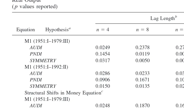
Table 4. Test Results of Null Hypotheses of Irrelevance of Distinctions Among Anticipated, Unanticipated Positive, and Unanticipated Negative Growth in M1 for Explaining Movement in Real Output

AUDI 0.0249 0.2378 0.2781 0.4979

PNDI 0.1454 0.0119 0.0037 0.0090

SYMMETRY 0.0317 0.0050 0.0018 0.0001

M1 (1951:I–1992:II)

AUDI 0.0286 0.0233 0.0364 0.1146

PNDI 0.0906 0.1671 0.1002 0.0369

SYMMETRY 0.0150 0.0135 0.0215 0.0195

Structural Shifts in Money Equationc

M1 (1951:I–1979:III)

AUDI 0.0248 0.1870 0.1619 0.1859

PNDI 0.1172 0.0001 0.0000 0.0000

SYMMETRY 0.0232 0.0001 0.0000 0.0000

M1 (1951:I–1992:II)

AUDI 0.1139 0.3654 0.0297 0.0615

PNDI 0.1404 0.0032 0.0040 0.0036

SYMMETRY 0.0701 0.0057 0.0001 0.0005

a

SYMMETRY-distinctions among anticipated, unanticipated positive, and unanticipated negative monetary policy change are irrelevant. Null hypothesis:bi

e_5b

AUDI-distinction between anticipated and unanticipated monetary policy change is irrelevant. Null hypothesis:bi e_5b

PNDI-distinction between unanticipated positive and unanticipated negative monetary policy change is irrelevant. Null hypothesis:bi

Forn54, regressions start from 1951:I. Asnincreases, regressions start at successively later dates.

c

money shocks did not affect output growth, and negative shocks had a highly significant

effect in reducing output (at least for the period 1951:I–1987:IV). The results of Cover

(1992), however, hold in an equation (which is not reported here), in which the anticipated

money terms were suppressed. Results for the period ending in 1987:IV, when

GM

u1

,

GM

u2

, and

GM

e

terms appear in the output equation, are similar to those for a period

ending in 1992:II, and over both periods, money was found to be non-neutral. The

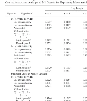
Table 5. Test of Null Hypotheses of Irrelevance of Unexpected Expansionary, Unexpected Contractionary, and Anticipated M1 Growth for Explaining Movement in Real GDP

Equation Hypothesisa

Lag Length

n54 n58 n512 n516

M1 (1951:I–1979:III)

Un. expansionary 0.1217 0.0190 0.0006 0.0004

Un. contractionary 0.3363 0.0187 0.0111 0.0013

Anticipated 0.0209 0.0079 0.0137 0.0017

With restriction

{Anticipated}b _{0.0792 0.1211 0.0650 0.1147}

Unanticipated 0.0551 0.0136 0.0015 0.0020

M1 (1951:I–1992:II)

Un. expansionary 0.0254 0.0119 0.0110 0.0075

Un. contractionary 0.0012 0.0141 0.0794 0.1555

Anticipated 0.0293 0.0405 0.1328 0.0506

With restriction

{Anticipated}b _{0.0420 0.1003 0.2078 0.1463}

Unanticipated 0.0024 0.0101 0.0267 0.0722

Structural Shifts in Money Equation M1 (1951:I–1979:III)

Un. expansionary 0.6226 0.0254 0.0019 0.0102

Un. contractionary 0.0001 0.0001 0.0001 0.0000

Anticipated 0.9771 0.0006 0.0012 0.0000

With restriction

{Anticipated}b _{0.8746 0.1367 0.0356 0.0172}

Unanticipated 0.0002 0.0347 0.0001 0.0003

M1 (1951:I–1992:II)

Un. expansionary 0.6757 0.0325 0.0228 0.0093

Un. contractionary 0.0158 0.0143 0.0018 0.0047

Anticipated 0.2334 0.4116 0.0355 0.0057

With restriction

{Anticipated}b _{0.4259 0.5456 0.1351 0.0736}

Unanticipated 0.0387 0.2138 0.0637 0.2654

a

For Un. Expansionary (unanticipated positive growth in M1), null hypothesis isbi u1₅

0,i50, 1, . . .n. For Un. Contractionary (unanticipated negative growth in M1), null hypothesis isbi

u2₅

inclusion of anticipated money in the output equation yielded positive money shocks

(

EXPANSIONARY

policy in Table 5) which were statistically significant. Anticipated

money was found, for the most part, to matter, and as noted in Table 5, did so more

strongly when a distinction between positive and negative money surprises was

recog-nized.

18

In Tables 2 and 3, for

n

5

4, it is reported that the null hypothesis that the sums of the

coefficients on positive money shocks, on negative money shocks, and on anticipated

money growth are significantly different from zero could not be rejected at the 0.05

level.

19

This result (not reported) was robust for various lag lengths and for both sample

periods. The implication of alternative specifications for the money equation will now be

briefly considered.

Alternative Specifications of the Equations

Intercept and slope dummy variables will now be introduced into the money equation to

account for structural change. This will have the effect of altering the measure of

expectations. Following Frydman and Rappoport (1987), in equation (1), the intercept is

allowed to differ before and after 1963:III and the coefficients of each of the variables

GM

t21

and

GM

t22

are allowed to differ before and after 1971:III.

20

It was found that

money equations estimated with these changes were much improved. Results under the

heading of “structural shifts in money equation” appear in Tables 4 and 5. There, it can

again be seen that for both sample periods,

SYMMETRY

was rejected over all

n

, whereas

AUDI could not be rejected except for

n

5

4. Other results were similar to those already

noted.

IV. Spread as Monetary Policy Indicator

In a number of recent papers, the importance of various interest-rate measures as

indicators of the stance of monetary policy has been emphasized. In this section, the

relevance of distinctions among unanticipated expansionary, unanticipated contractionary,

and anticipated policy, when the indicator of monetary policy is taken to be spread, is

investigated.

21

_{Spread was regressed on four-lagged values of itself and on four-lagged}

values of a number of economic variables. These variables were

GM

,

GY

,

GB

,

UR

,

FEBS

,

18_{Cover (1992) noted the non-neutrality of money for the period 1951:I–1987:IV. However, because the} coefficients on theGMt

1_{terms were of the wrong sign in the presence of anticipated money terms, Cover’s}

preferred regression equation is one in which anticipated money growth terms were excluded. Note that the main finding of Cover concerning an asymmetry between positive and negative money shocks in explaining movement in output continues to be confirmed in this paper.

19_{Cover (1992) also reported a similar result when anticipated money was included in the output equation} [see Cover (1992, Tables VI and VII, pp. 1273, 1275)]. He found that the sums of coefficients on the positive shocks (SUM(POS)) and on negative shocks (SUM(NEG)) were not statistically significant at the 0.05 level. When anticipated money terms did not appear in the output equation, Cover (1992, pp. 1269–70) found that SUM(NEG) was statistically significant at the 0.01 level (and thatSUM(POS) was insignificant).

and GDP inflation (

GDINF

).

22

GY

,

GB

, and

GDINF

were not statistically significant for

1949:II–1992:II. Thus, four-lagged values of

GM

,

UR

, and

FEBS

appear along with

four-lagged values of spread in the forecasting equation for spread.

To begin with, four-lagged values of the dependent variable,

GY

t

, and current and

four-lagged values of anticipated change, and positive and negative innovations in spread

appear in the output equation.

23

_{A positive (negative) surprise in spread indicates that}

spread was greater (less) than expected and, hence, that monetary policy was more

contractionary (expansionary) than expected. The coefficients on the monetary policy

variables should be negative (at least at first). To avoid confusion,

MPI

t

e

_,

MPI

t

u1

_{, and}

MPI

t

u2

_{refer to anticipated, unexpected expansionary, and unexpected contractionary}

policy, respectively.

The results of joint estimation of equations for spread and for output for the period

1950:II–1992:II appear in Tables 6 and 7, respectively. Sets I and II are again estimates

of equations (1) and (2), and of equations (1) and (3). In the spread equations in Table 6,

it can be seen that increases in the rate of money growth and in the budget surplus tended

22_{Four-lagged values of each of these variables were retained in the equation explaining spread only if they} were jointly significant at the .05 level or stronger. This was the method employed by Mishkin (1982, p. 30). 23_{Four lags in the spread terms are indicated by AIC from examination of the output equation before} applying a joint estimation. The residuals of the output equation do not show first-order or higher-order serial correlation.

Table 6. Monetary Policy Equations with Spread as Monetary Policy Indicator: Nonlinear Joint Estimation 1950:II–1992:II

(standard errors in parentheses)

Set I Set II

Variable Coefficient pValue Coefficient pValue

Constant 0.200 (0.077) 0.0098 0.147 (0.099) 0.1386

MPI{1} 0.630 (0.055) 0.0000 0.690 (0.073) 0.0000

MPI{2} 20.038 (0.067) 0.5739 20.083 (0.089) 0.3512

MPI{3} 0.076 (0.067) 0.2556 0.066 (0.089) 0.4544

MPI{4} 0.057 (0.053) 0.2885 0.168 (0.078) 0.0313

UR{1} 20.004 (0.047) 0.9331 20.122 (0.061) 0.0445

UR{2} 0.118 (0.080) 0.1422 0.272 (0.110) 0.0136

UR{3} 20.336 (0.085) 0.0001 20.356 (0.112) 0.0015

UR{4} 0.212 (0.048) 0.0000 0.191 (0.061) 0.0018

FEBS{1} 0.427 (0.109) 0.0001 0.320 (0.135) 0.0176

FEBS{2} 20.036 (0.133) 0.7896 0.182 (0.163) 0.2659

FEBS{3} 20.485 (0.133) 0.0003 20.597 (0.180) 0.0008

FEBS{4} 0.170 (0.127) 0.1830 0.167 (0.155) 0.2823

GM{1} 0.038 (0.024) 0.1200 0.071 (0.028) 0.0112

GM{2} 20.015 (0.024) 0.5376 20.048 (0.031) 0.1141

GM{3} 20.014 (0.025) 0.5834 0.002 (0.030) 0.9214

GM{4} 0.086 (0.022) 0.0002 0.057 (0.027) 0.0353

Std. error 0.307 0.301

DW 1.933 1.957

R2 _{0.534 0.549}

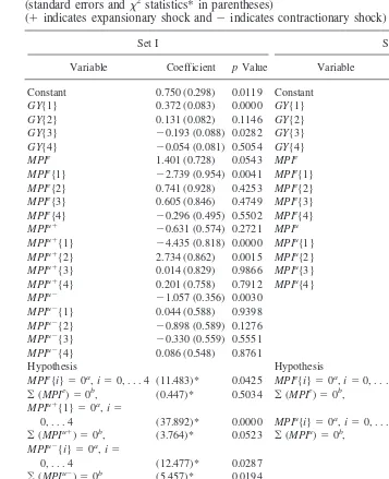
Table 7. Output Equations with Spread as Monetary Policy Indicator (MPI): Nonlinear Joint Estimation 1950:II–1992:II

(standard errors andx2_{statistics* in parentheses)}

(1indicates expansionary shock and2indicates contractionary shock)

Set I Set II

Variable Coefficient pValue Variable Coefficient pValue

Constant 0.750 (0.298) 0.0119 Constant 1.216 (0.288) 0.0000

GY{1} 0.372 (0.083) 0.0000 GY{1} 0.210 (0.085) 0.0137

GY{2} 0.131 (0.082) 0.1146 GY{2} 0.102 (0.083) 0.2178

GY{3} 20.193 (0.088) 0.0282 GY{3} 20.169 (0.085) 0.0469

GY{4} 20.054 (0.081) 0.5054 GY{4} 20.062 (0.082) 0.4529

MPIe _{1.401 (0.728) 0.0543 MPI}e _{1.676 (0.741) 0.0237}

MPIe_{{1} 22.739 (0.954) 0.0041 MPI}e_{{1} 21.981 (0.877) 0.0238}

MPIe_{{2} 0.741 (0.928) 0.4253 MPI}e_{{2} 0.081 (0.795) 0.9185}

MPIe_{{3} 0.605 (0.846) 0.4749 MPI}e_{{3} 20.591 (0.760) 0.4365}

(5)-test of the null hypothesis that the coefficients onMPIe

(MPIu1

,MPIu2

, orMPIu

) terms are jointly zero.

b_x2

(1)-test of the null hypothesis that the sum of the coefficients on theMPIe

(MPIu1

(10)-test of joint pairwise equality and of joint triple-wise equality, respectively, of coefficients on variables indicated.

d_x2

(1)-test andx2

to raise spread one quarter later, after which time the effect was eroded, and a rise in the

unemployment rate tended to reduce spread after three quarters followed by a reversal in

the fourth quarter. In the output equation in Table 7, the null hypothesis that distinctions

among anticipated, unanticipated positive, and unanticipated negative changes in spread is

irrelevant in explaining growth in output (

SYMMETRY

) was rejected.

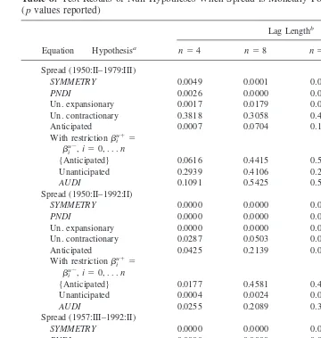
The effects of increasing

n

for the period ending in 1992:II, and for a period ending in

1979:III, are reported in Table 8. Also, results are presented for a period starting in

1957:III. This sample period was included because it matches the period for which results

were available on the federal funds rate as the measure of monetary policy. From Table

8, it can be seen that as lag length increased in the spread variables, the null hypothesis

of equality of coefficients on

MPI

u1

,

MPI

u2

, and

MPI

e

continued to be rejected at the 0.01

level.

24

Expansionary monetary policy, signaled by spread, usually had a statistically

signifi-cant effect on output in Table 8. The exception was for the sample ending in 1979:III with

n

5

16. It is interesting that contractionary monetary policy signaled by spread was not

usually quite as potent, especially for the sample ending in 1979:III. Consistent with the

M1 results, spread as an indicator of monetary policy reinforces the conclusion that

asymmetries among the effects of anticipated, expansionary unanticipated, and

contrac-tionary unanticipated monetary policy on aggregate output are of some empirical

impor-tance.

25

V. Federal Funds Rate as Monetary Policy Indicator

The use of change in the federal funds rate as a monetary policy indicator provides an

opportunity to test a stimulative/contractionary distinction in the effect on output.

Antic-ipated changes in the federal funds rate are divided into positive (anticAntic-ipated

contraction-ary) and negative (anticipated stimulative) components,

MPI

e2

and

MPI

e1

, respectively.

The output equation is given by:

GY

t

5

a

0

1

O

It is now possible to test the following two hypotheses:

26

H

₀

(SC):

No stimulative/contractionary asymmetry given by

b

_ie1

5

b

_ie2

and

b

_iu1

5

b

_iu2

,

i

5

1, . . .

n

.

H

₀

(AU):

No anticipated/unanticipated asymmetry given by

b

_ie1

5

b

_iu1

and

b

_ie2

5

b

_iu2

,

i

5

1, . . .

n

.

24_{As a check for robustness, an alternative specification of the spread equation was tried in which four lags} of real growth (GY) and of inflation (GDINFL) were added to those listed in the spread equation in Table 6. Results were found to be very similar to those given in Tables 7 and 8 (concerning effects of spread as MPI) and, thus, are not reported here.

25_{In contrast to results when monetary policy was measured by growth in M1, results in Table 8 suggest that} anticipated change in spread has, at best, only marginal effects on output (except whenn54).

Table 8. Test Results of Null Hypotheses When Spread is Monetary Policy Indicator

SYMMETRY 0.0049 0.0001 0.0001 0.0000

PNDI 0.0026 0.0000 0.0000 0.0000

Un. expansionary 0.0017 0.0179 0.0223 0.4890

Un. contractionary 0.3818 0.3058 0.4120 0.0082

Anticipated 0.0007 0.0704 0.1384 0.4302

With restrictionbiu

1₅ biu

2_{,i50, . . .n}

{Anticipated} 0.0616 0.4415 0.5884 0.9426

Unanticipated 0.2939 0.4106 0.2190 0.4695

AUDI 0.1091 0.5425 0.5453 0.9406

Spread (1950:II–1992:II)

SYMMETRY 0.0000 0.0000 0.0000 0.0000

PNDI 0.0000 0.0000 0.0000 0.0000

Un. expansionary 0.0000 0.0000 0.0000 0.0000

Un. contractionary 0.0287 0.0503 0.0326 0.0262

Anticipated 0.0425 0.2139 0.0821 0.0801

With restrictionbiu

1₅ biu

2_{,i50, . . .n}

{Anticipated} 0.0177 0.4581 0.4642 0.6535

Unanticipated 0.0004 0.0024 0.0123 0.0527

AUDI 0.0255 0.2089 0.3646 0.5426

Spread (1957:III–1992:II)

SYMMETRY 0.0000 0.0000 0.0000 0.0000

PNDI 0.0000 0.0000 0.0000 0.0000

Un. expansionary 0.0000 0.0000 0.0000 0.0000

Un. contractionary 0.0053 0.0002 0.0004 0.0000

Anticipated 0.3477 0.3800 0.2576 0.1083

With restrictionbiu

1₅ biu

2_{,i50, . . .n}

{Anticipated} 0.2301 0.2846 0.5347 0.5322

Unanticipated 0.0009 0.0085 0.2314 0.0684

AUDI 0.0547 0.2173 0.5137 0.5372

a

SYMMETRY-distinctions among anticipated, unanticipated positive, and unanticipated negative monetary policy are irrelevant. Null hypothesis:bi

e_5b

AUDI-distinction between anticipated and unanticipated monetary policy is irrelevant. Null hypothesis:bi e_5b

PNDI-distinction between unanticipated positive, and unanticipated negative monetary policy is irrelevant. Null hypothesis:

bi u1_5b

i u2

,i50, 1, . . .n.

Un. expansionary refers to unanticipated negative spread (null hypothesis isbi u1₅

0,i50, 1, . . .n). Un. contractionary refers to unanticipated positive spread (null hypothesis isbi

u2₅

0,i50, 1, . . .n). Anticipated-null hypothesis isbi

e₅

0,i50, 1, . . .n. Null hypothesis for {Anticipated}:bi

e₅

The change in the federal funds rate is now regressed on four-lagged values of itself

and on four-lagged values of a number of economic variables which have been previously

introduced.

27

The variables tried on the righthand side of equation (1) as explanatory

variables include four lags of the variables

GM

,

GY

,

UR

,

FEBS

, and

GDINF

. Four-lagged

values of each of these variables were retained in the equation explaining spread only if

they were jointly significant at the .05 level or stronger. It was found that the lagged

dependent variable,

GY

, and

GDINF

were statistically significant.

In the output equation, two-lagged values of the dependent variable,

GY

, and current

and five-lagged values of anticipated and unanticipated positive and negative innovations

in the change in the federal funds rate appear on the basis of AIC. The current and lagged

value of the change in the T-bill rate (

DTBR

) are also included as explanatory variables

in the output equation.

28

Innovations in the change in the federal funds rate should be

negatively associated with real output growth (at least, at first).

The federal funds rate equation and the output equation were jointly estimated and the

results are presented in Tables 9 and 10. Set I refers to joint estimation of equations (1)

and (2

9

), and Set II refers to joint estimation of equations (1) and (3). In the federal funds

equations, it can be seen that increases in the rate of real growth raised the change in the

federal funds rate for several quarters, and that an increase in the rate of inflation had the

same effect for about two quarters.

27_{The level of the federal funds rate is non-stationary and the change in the federal funds rate is stationary.} 28_{As emphasized by Bernanke and Blinder (1992), when interpreting movement in the federal funds rate, it} helps to know the current level of market rates of interest.

Table 9. Monetary Policy Equations with Change in Federal Funds Rate as Monetary Policy Indicator: Nonlinear Joint Estimation 1957:III–1992:II

(standard errors in parentheses)

Set I Set II

Variable Coefficient pValue Coefficient pValue

Constant 21.122 (0.199) 0.0000 20.726 (0.244) 0.0029

MPI{1} 0.069 (0.059) 0.2402 0.063 (0.084) 0.4517

MPI{2} 20.300 (0.066) 0.0000 20.356 (0.082) 0.0000

MPI{3} 0.034 (0.052) 0.5138 0.087 (0.088) 0.3234

MPI{4} 0.027 (0.054) 0.6103 0.018 (0.080) 0.8172

GY{1} 0.294 (0.059) 0.0000 0.373 (0.095) 0.0000

GY{2} 0.116 (0.054) 0.0328 0.154 (0.089) 0.0853

GY{3} 0.216 (0.052) 0.0000 0.119 (0.078) 0.1255

GY{4} 0.088 (0.050) 0.0810 0.002 (0.065) 0.9716

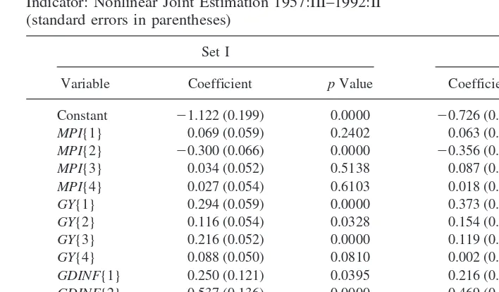
GDINF{1} 0.250 (0.121) 0.0395 0.216 (0.131) 0.0993

GDINF{2} 0.537 (0.136) 0.0000 0.469 (0.167) 0.0049

GDINF{3} 20.326 (0.124) 0.0089 20.039 (0.138) 0.7738

GDINF{4} 0.009 (0.101) 0.9193 20.396 (0.167) 0.0178

Std. error 0.978 0.949

DW 1.930 1.981

R2 _{0.238 0.276}

Table 10. Output Equations with Change in Federal Funds Rate as Monetary Policy Indicator (MPI): Nonlinear Joint Estimation 1957:III–1992:II

(standard errors andx2_{statistics* in parentheses)}

(1indicates expansionary policy and2indicates contractionary policy)

Set I Set II

Variable Coefficient pValue Variable Coefficient pValue

Constant 0.223 (0.199) 0.0000 Constant 0.285 (0.170) 0.0941

GY{1} 0.367 (0.143) 0.0102 GY{1} 0.554 (0.225) 0.0137

GY{2} 0.325 (0.157) 0.0390 GY{2} 0.050 (0.208) 0.8086

DTBR 0.818 (0.190) 0.0000 DTBR 0.597 (0.188) 0.0014

DTBR{1} 0.121 (0.218) 0.5779 DTBR 0.203 (0.201) 0.3107

MPIe1 _{21.152 (0.417) 0.0058 MPI}e _{21.298 (0.506) 0.0103}

MPIe1_{{1} 0.388 (0.443) 0.3816 MPI}e_{{1} 0.618 (0.555) 0.2656}

MPIe1_{{2} 20.429 (0.304) 0.1582 MPI}e_{{2} 20.735 (0.458) 0.1086}

MPIe1_{{3} 20.140 (0.282) 0.6190 MPI}e_{{3} 0.350 (0.410) 0.3939}

MPIe1_{{4} 20.096 (0.266) 0.7171 MPI}e_{{4} 20.147 (0.261) 0.5708}

MPIe1_{{5} 0.010 (0.237) 0.9663 MPI}e_{{5} 20.117 (0.155) 0.4499}

MPIe2 _{20.844 (0.485) 0.0822 MPI}u _{20.131 (0.156) 0.3990}

MPIe2_{{1} 21.431 (0.611) 0.0191 MPI}u_{{1} 20.045 (0.185) 0.8041}

MPIe2_{{2} 1.574 (0.508) 0.0019 MPI}u_{{2} 20.671 (0.232) 0.0039}

MPIe2_{{3} 20.340 (0.401) 0.3956 MPI}u_{{3} 0.247 (0.279) 0.3747}

MPIe2_{{4} 0.334 (0.396) 0.3986 MPI}u_{{4} 20.278 (0.215) 0.1948}

MPIe2_{{5} 20.678 (0.345) 0.0496 MPI}u_{{5} 20.200 (0.138) 0.1477}

MPIu1 _{20.285 (0.207) 0.1691 Hypothesis}

MPIu1_{{1} 20.128 (0.222) 0.5633 MPI}e_{i}50a_{,i50, . . . 5 (11.459)* 0.0751}

MPIu1_{{2} 20.507 (0.205) 0.0136 ¥(MPI}e₎₅₀b_{, (7.985)* 0.0047}

MPIu1_{{3} 20.414 (0.231) 0.0733 MPI}u_{i}50a_{,i50, . . . 5 (26.054)* 0.0002}

MPIu1_{{4} 0.128 (0.190) 0.4987 ¥(MPI}u₎₅₀b_{, (12.675)* 0.0003}

MPIu1_{{5} 0.011 (0.155) 0.9401}

MPIu2 _{20.283 (0.186) 0.1288 MPI}e_{i}5MPIu_{i}a_{, (7.771) 0.2553}

MPIu2_{{1} 20.053 (0.191) 0.7779 ¥(MPI}e_)5¥(MPIu₎b _{(0.347) 0.5559}

MPIu2_{{2} 20.326 (0.175) 0.0626}

MPIu2_{{3} 20.185 (0.201) 0.3576 Std. error 0.744}

MPIu2_{{4} 0.122 (0.176) 0.4856 DW 2.028}

MPIu2_{{5} 20.535 (0.170) 0.0016 R}2 _0.431

Hypothesis

MPIe1_{i}50a_{, (14.929)* 0.0208 ¥(MPI}e1₎₅₀b_{, (7.969)* 0.0047}

MPIe2_{i}50a_{, (19.866)* 0.0029 ¥(MPI}e2₎₅₀b_{, (5.957)* 0.0146}

MPIu1_{i}50a_{, (17.419)* 0.0078 ¥(MPI}u1₎₅₀b_{, (10.481)* 0.0012}

MPIu2_{i}50a_{, (23.707)* 0.0005 ¥(MPI}u2₎₅₀b_{, (14.168)* 0.0001}

MPIe1_{i}5MPIe2_{i}a _{(19.194)* 0.0038 ¥(MPI}e1_)5¥(MPIe2₎b _{(0.001)* 0.9660}

MPIu1_{i}5MPIu2_{i}a

i50, 1 . . . 5 (7.763)* 0.2559 ¥(MPIu1_)5¥(MPIu2₎b _{(0.038)* 0.8450}

SC: No stimulative/contractionary:MPIe1_{i}5MPIe2_{{i} andMPI}u1_{i}5MPIu2_{i}c

(25.259)* 0.0136

AU: No anticipated/unanticipated:MPIe1_{i}5MPIu1_{{i} andMPI}e2_{i}5MPIu2_{i}c

(20.913)* 0.0516

Std. error 0.625

DW 1.994

R2 _0.602

a_x2

(6)-test of the null hypothesis for coefficients on variables indicated.

b_x2

(1)-test of the null hypothesis for coefficients on variables indicated.

c_x2

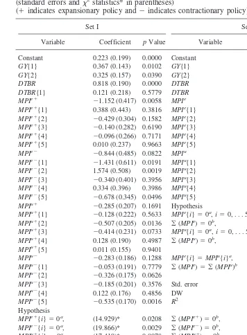
In Table 10, it is reported, based on exclusion tests, that each of the four components

of policy had statistically significant effects on output. The cumulative effects were also

each found to be statistically significant. This latter result is different from that obtained

when MPI was measured by growth in M1.

Results on the no stimulative/contractionary asymmetry (

SC

) and no anticipated/

unanticipated (

AU

) hypotheses are reported at the bottom of Table 10. It was found that

SC

was rejected at the 0.0136 level. This result would seem to be based on the finding of

asymmetry in anticipated policy between stimulative and contractionary actions. This

follows, as the null hypothesis of

b

_ie1

5

b

_ie2

,

i

5

0, 1 . . . 5 was rejected with

p

value

0.0208, compared to failure to reject the null hypothesis of

b

_iu1

₅

_b

i u2

,

i

5

0, 1, . . . 5. In

addition, it will be noted from Set II, that the exclusion test for anticipated money had a

p

value of only 0.0751. Thus, recognition of an asymmetry in anticipated policy would

again seem to be of importance to results. In Table 10,

AU

was rejected at the 0.0516 level.

The results discussed here for

n

5

5 generally held for longer lag lengths and are

reported in Table 11.

29

For the purpose of comparison with the results obtained in the

earlier part of the paper, results are presented in Table 12 for the federal funds rate, in

which an asymmetry in anticipated policy was not recognized (these results can be

contrasted with those for spread summarized in Table 8).

In Table 11, asymmetries are to be found in both stimulative versus contractionary

policy, and in anticipated versus unanticipated effects. For changes in the federal funds

rate, as a measure of monetary policy, it would seem that an asymmetry in the effects on

output of anticipated policy between stimulative and contractionary components is of

some empirical importance.

To illustrate these asymmetries, a simple five-variable VAR(

GY

,

MPI

u2

,

MPI

u1

,

MPI

e2

,

MPI

e1

) was estimated and impulse response functions for

GY

obtained.

30

The

impulse responses of growth in GDP (

GY

) to one-standard-error shocks to

MPI

u2

and

MPI

u1

are shown in Figure 1, and to

MPI

e2

and

MPI

e1

in Figure 2. In Figure 1, the

negative effect of unanticipated contractionary policy was initially somewhat larger in

absolute value than the positive effect of unanticipated stimulative policy. Both effects on

GY

fluctuated and decayed fast (with eight quarters). In Figure 2, the negative effect of

anticipated contractionary policy was larger in absolute value in the first two quarters than

the positive effect of anticipated stimulative policy.

MPI

e2

showed a positive effect after

two quarters. Thus, it seems that anticipated contractionary policy has a relatively large,

but short-lived, negative effect on

GY

. The impulse responses from the VAR are

consis-29_{Results are not reported for a period ending in 1979:III because there was an inadequate number of degrees} of freedom available for test statistics. As a check for robustness for the results over the period 1957:III–1992:II, an alternative specification of the federal funds rate equation in Table 9 was tried. In addition to four lags ofGY and ofGDINFL, four lags each ofUR,FEBS, andGMwere added as explanatory variables in the federal funds rate equation. The main difference in results concerned unanticipated policy.AUwas more likely to be rejected, withpvalues that the anticipated/unanticipated distinction not being relevant (H0(AU):bie

1₅

the hypothesis of no asymmetry in unanticipated policy (H0:biu

1₅ biu

2_{) was also more likely to be rejected with}

pvalues 0.8628 (n55), 0.0061 (n58), 0.0000 (n512), and 0.0000 (n516). Results for asymmetry in anticipated policy were similar to those already reported. Given limitations of space, these results are not reported here.

30_MPIu2_,

MPIu1_,

MPIe2_,

MPIe1_{were obtained for change in the federal funds rate implied by Set I in}

Table 11. Test Results of Null Hypotheses with Federal Funds Rate as Measure of Monetary Policy for 1957:III–1992:II

(pvalues reported;x2_{( )-statistics in parentheses)}

Hypothesis Lag Length

n55 n58 n512 n516

No Anticipated Expansionary Effect Ho:bie

1_{50,i50, 1 . . .n}a

0.0208 (14.929) 0.0074 (22.483) 0.0683 (21.236) 0.0038 (36.534) Ho:¥bie

1_{overi50, 1 . . .n}b

0.0047 (7.969) 0.0001 (14.414) 0.0019 (9.576) 0.0442 (4.047) No Anticipated Contractionary Effect

Ho:bie

2_{50,i50, 1 . . .n}a

0.0029 (19.866) 0.0011 (27.523) 0.0019 (32.570) 0.0191 (31.151) Ho:¥bie

2_{overi50, 1 . . .n}b

0.0146 (5.957) 0.0014 (10.093) 0.0064 (7.428) 0.2394 (1.383) No Unanticipated Expansionary Effect

Ho:biu

1_{50,i50, 1 . . .n}a

0.0078 (17.419) 0.0157 (20.374) 0.0083 (28.259) 0.0013 (39.821) Ho:¥biu

1_{overi50, 1 . . .n}b

0.0012 (10.481) 0.0001 (14.310) 0.0002 (13.265) 0.0146 (5.961) No Unanticipated Contractionary Effect

Ho:biu

2_{50,i50, 1 . . .n}a

0.0005 (23.707) 0.0001 (33.439) 0.0019 (32.585) 0.0017 (39.039) Ho:¥biu

2_{overi50, 1 . . .n}b

0.0001 (14.168) 0.0001 (14.765) 0.0037 (8.425) 0.1335 (2.250) No Asymmetry in Anticipated Policy

Ho:bie

1₅ bie

2_{50,i50, 1 . . .n}a

0.0038 (19.194) 0.0178 (20.002) 0.0329 (23.811) 0.0064 (34.863) Ho:¥bie

1_5¥ bie

2_overi50,

1 . . .nb

0.9660 (0.001) 0.7835 (0.075) 0.8094 (0.068) 0.9297 (0.007) No Asymmetry in Unanticipated Policy

Ho:biu

1₅ biu

2_{50,i50, 1 . . .n}a

0.2559 (7.763) 0.2693 (11.094) 0.1216 (19.047) 0.0033 (37.012) Ho:¥biu

1_5¥ biu

2_overi50,

1 . . .nb

0.8450 (0.038) 0.9310 (0.007) 0.8966 (0.152) 0.4404 (0.595) No Stimulative/Contractionary Asymmetry

0.0136 (25.259) 0.0538 (28.573) 0.0062 (47.459) 0.0003 (69.193) No Anticipated/Unanticipated Asymmetry

0.0516 (20.913) 0.0726 (27.350) 0.0964 (35.743) 0.0470 (48.906)

a_x2

test withn11 degrees of freedom.

b_x2

test with one degree of freedom.

c_x2

tent with the results noted in Table 11, concerning an asymmetry in anticipated policy

between stimulative and contractionary effects.

VI. Conclusion

For monetary policy measured by change in the federal funds rate, an asymmetry in the

effects of anticipated expansionary and anticipated contractionary monetary policy on

output was found. The null hypothesis of no asymmetry in stimulative/contractionary

policy was rejected. Anticipated expansionary, anticipated contractionary, unanticipated

expansionary, and unanticipated contractionary monetary policy were each found to have

statistically significant effects on output. Each of the four components of monetary policy

were also found to have statistically significant cumulative effects on output.

Table 12. Test Results of Null Hypotheses When Federal Funds Rate is Monetary Policy Indicator. Asymmetry in Anticipated Policy not Recognized (bi

e1_5b

SYMMETRY 0.3598 0.0000 0.0000 0.0000

PNDI 0.2632 0.0000 0.0000 0.0000

Un. expansionary 0.8846 0.0063 0.0930 0.0000

Un. contractionary 0.0195 0.0005 0.0001 0.0000

Anticipated 0.6415 0.4207 0.9365 0.0011

With restrictionbiu

1₅ biu

2_,i

50, . . .n

{Anticipated} 0.6014 0.9028 0.1590 0.4211

Unanticipated 0.5689 0.0192 0.0030 0.0169

AUDI 0.4260 0.6435 0.2691 0.5539

Federal Funds (1957:III–1992:II)

SYMMETRY 0.2383 0.1140 0.0558 0.0118

PNDI 0.3147 0.1322 0.0133 0.0004

Un. expansionary 0.1421 0.0585 0.0028 0.0024

Un. contractionary 0.0003 0.0003 0.0015 0.0000

Anticipated 0.0357 0.0055 0.0855 0.0716

With restrictionbiu

1₅ biu

2_,i

50, . . .n

{Anticipated} 0.0751 0.0245 0.4450 0.3898

Unanticipated 0.0002 0.0004 0.0000 0.0006

AUDI 0.2553 0.3239 0.6074 0.8436

a

SYMMETRY-distinctions among anticipated, unanticipated positive, and unanticipated negative monetary policy are irrelevant. Null hypothesis:bi

e_5b

AUDI-distinction between anticipated and unanticipated monetary policy is irrelevant. Null hypothesis:bi e_5b

i u

,i50, 1, . . .n.

PNDI-distinction between unanticipated positive, and unanticipated negative monetary policy is irrelevant. Null hypothesis:

bi u1_5b

i u2

,i50, 1, . . .n.

Un. Expansionary refers to unanticipated negative change in federal funds rate (null hypothesis isbi u1₅

0,i50, 1, . . .n). Un. Contractionary refers to unanticipated positive change in federal funds rate (null hypothesis isbi

u2₅

0,i50, 1, . . .n). Anticipated-null hypothesis isbi

e₅

0,i50, 1, . . .n. Null hypothesis for {Anticipated}:bi

e₅

For different measures of monetary policy, different specifications of the monetary

policy and output equations, and over different sample periods, distinctions among

positive innovations, negative innovations, and anticipated monetary policy change were

found to be relevant for explaining movement in real output. Unanticipated expansionary

monetary policy was found to be just as likely to have a statistically significant effect on

output as unanticipated contractionary monetary policy. In addition, recognition of

asym-metries in anticipated and unanticipated monetary policy between stimulative and

con-tractionary components made the finding of neutrality of money less likely.

Figure 1. Impulse response of GDP to money shocks.