Ž .
Energy Economics 22 2000 549]568
Are oil markets chaotic? A non-linear
dynamic analysis
Epaminondas Panas
U, Vassilia Ninni
Athens Uni¨ersity of Economics and Business, 76 Patission St., Athens 104 34, Greece
Abstract
The analysis of products’ price behaviour continues to be an important empirical issue. This study contributes to the current literature on price dynamics of products by examining for the presence of chaos and non-linear dynamics in daily oil products for the Rotterdam and Mediterranean petroleum markets. Previous studies using only one invariant, such as the correlation dimension may not effectively determine the chaotic structure of the underlying time series. To obtain better information on the time series structure, a framework is developed, where both invariant and non-invariant quantities were also examined. In this paper various invariants for detecting a chaotic time series were analysed along with the associated Brock’s theorem and Eckman]Ruelle condition, to return series for the prices of oil products. An additional non-invariant quantity, the BDS statistic, was also examined. The correlation dimension, entropies and Lyapunov exponents show strong evidence of chaos in a number of oil products considered.Q2000 Elsevier Science B.V. All rights reserved.
Keywords: Petroleum products; Correlation dimension; Entropy; Lyapunov exponent; Non-linear dynamic; Chaos
1. Introduction
Ž .
In the last 10 years since the publications of Frank and Stengos 1989 , who found evidence of non-linear structure in the rates of return of gold and silver, economists have been engaged in an attempt to detect non-linear structure in
Ž .
economic time series. Various authors, such as Frank and Stengos 1989 ,
U
Corresponding author.
Ž .
E-mail address:[email protected] E. Panas .
0140-9883r00r$ - see front matterQ2000 Elsevier Science B.V. All rights reserved.
Ž .
Ž . Ž . Ž .
Scheinkman and LeBaron 1989a,b , Blank 1991 , Hsieh 1991 , DeCoster et al.
Ž1992 , Yang and Brorsen 1993 , Fang et al. 1994 , Kohzadi and Boyd 1995 , have. Ž . Ž . Ž .
found strong evidence of non-linear structure and, in particular, of chaotic struc-ture in the ‘behaviour of economic’ time series.
In particular, the empirical analysis of the economic time series in a non-linear framework is important for at least three principal reasons. First, the effort devoted to study time series reflects the fact that non-linearities convey informa-tion about the structure of the series under study. Second, these non-linearities provide insight into the nature of the process governing the structure of these time series. Third, in the absence of information about the structure of these time series it is difficult to distinguish the stochastic from the chaotic process.
Ž . Ž .
Various authors, e.g. DeCoster et al. 1992 , Yang and Brorsen 1993 , have examined for chaos in economic data based only on one invariant. More specifi-cally, the correlation dimension technique has been used. This technique, however,
can only give an unreliable indication of chaos if for example the Eckmann]Ruelle
Ž1992 condition is not satisfied..
This non-reliability is increased given that, in almost all empirical applications the choice of a time delay is arbitrary. More specifically, in dealing with chaotic behaviour the problem posed in time series analysis is the determination of the following invariants: fractal dimension; entropies; and Lyapunov exponents. From
4
the knowledge of economic time series Zt, ts1,2,...,n, we can produce a
Ž . Ž .
reconstructed phase-space or embedding space by the method of Takens 1981 ,
Z ,t Ztqt, Ztq2t,...,ZtqŽmy1.t4, having the same invariant structure as Zt, ts
4
1,2,...,n. In almost all empirical results the time delay,t, is often chosen arbitrarily.
The specification of the time delay is of central importance, since the choice of t
influences the values of the invariants. For this reason, in this paper, we focus our
attention on how to choose t. In this fashion we will address the issue of the
quality of reconstructed time series.
There are a variety of criteria or methods that can be used to examine the chaotic behaviour of time series. There are advantages and disadvantages to each of these criteria and there is no obviously superior approach. These criteria are:
Ž .i correlation dimension; ii entropy; iii maximal Lyapunov exponent; ivŽ . Ž . Ž .
Ž . Ž .
Eckmann]Ruelle condition; v Brocks or residual test theorem; and vi BDS
statistic test.
The importance of these criteria in examining the chaotic structure lies not only in their usefulness in analysing the non-linear structure but also in their relevance and potential utility to distinguish between stochastic behaviour and deterministic chaos. It is, therefore, essential that a careful investigation be made into the
validity of these criteria } towards which goal this paper is a small first step. An
( )
E. Panas, V. NinnirEnergy Economics 22 2000 549]568 551
Ž .
NAPHTHA; MOGAS PREM. 0.15 GrL; JET FUELrKERO ; GASOIL 0.2%
SULFUR; FO 3.5% SULFUR; FO 1.0% SULFUR; MOGAS REG UNL; MOGAS PREM. UNL 95 for the Rotterdam and Mediterranean markets.
This paper is organised as follows. Following this introductory section, we present our empirical results in Section 2. Finally our main concluding remarks are presented in Section 3.
2. Empirical results
We use two major petroleum markets, namely those of Rotterdam and the Mediterranean. The sample consists of the daily prices of different oil products from 4 January 1994 to 7 August 1998, resulting in 1161 observations. All prices were collected from OPEC.
Let pt be the oil product price at date t then
Ž . Ž .
Ztslog ptrpty1 1
is the daily log price relatives.
Ž .
Thus, the transformed data given by Eq. 1 are rates of return. In this paper we will study the daily behaviour of oil product prices, using the scalar time series
ZtslogŽptrpty1. 4
Chaos tests can be conducted on the original data directly without involving filters. However, in the approach taken here we will use both the original as well as
Ž . Ž .
the filtered data. The filters used in this paper are obtained by AR k -GARCH p,q models.
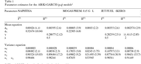
There are many different types of GARCH models used in finance. In this study we determine the ‘best’ among the various types of GARCH models by minimising Akaike’s information criterion. Table 1 reports the results of fitting the ‘best’
GARCH model to each oil product return. The table reports t-statistics using
robust standard errors in parentheses below each coefficient estimate, see
Boller-Ž .
slev and Wooldridge 1992 . It follows from Table 1 that:
1. Except for the Naphtha series in the Rotterdam market, the return series are all positively skewed, that is, the distribution of these series is skewed to the right. The skewness results in Table 1 show that the distributions of all daily returns are significantly skewed. The kurtosis coefficients are in all cases significantly leptokurtic. The combination of a significant asymmetry and leptokurtosis indicates that oil product returns are non-normally distributed.
Ž .
By inspecting Table 1, we see that the BJ Bera]Jarque test rejects the null
hypothesis of a normal distribution for both the Rotterdam and Mediterranean markets. These results imply that returns on oil products are not normally distributed for both Rotterdam and Mediterranean markets, and according to
Ž .
()
Parameter estimates for the AR K -GARCH p,q models
Ž .
Parameters NAPHTHA MOGAS PREM. 0.15 GrL JET FUELrKERO GASOIL 0.2%
SULFUR
ŽI. ŽI. ŽI. ŽI. ŽI. ŽI. ŽI. ŽI.
I II I II I II I II
Mean equation
Ž . Ž . Ž . Ž . Ž . Ž . Ž . Ž .
f0 0.00026 1.1 0.00395 2.6 y0.00005 3.9 0.0003 2.2 0.00355 2.6 0.002574 2.9 0.00383 2.6 0.00207 2.34
Ž . Ž .
f1 0.32674 10.04 0.22305 6.8
Ž . Ž . Ž . Ž . Ž .
g y0.28877 2.12 y0.28239 2.51y11.4113 2.85 y0.28803 2.6 y8.9985 2.31
l 0.5 0.5 2 0.5 2
Variance equation
a0 0.000003 0.000028 0.000039 0.00004 0.00004 0.00006 0.000006 0.000007
Ž . Ž . Ž . Ž . Ž . Ž . Ž . Ž .
a1 0.08082 2.1 0.0858 2.3 0.17853 3.0 0.0245 3.75 0.10797 3.3 0.00738 2.9 0.10500 2.9 0.08378 3.2
Ž . Ž . Ž . Ž . Ž . Ž . Ž . Ž .
a2 0.90524 19.03 0.89684 17.2 0.69802 9.2 0.51495 5.59 0.87744 30.9 0.90431 35.7 0.87542 32.2 0.89236 31.76
a1qa2 0.98606 0.98264 0.87655 0.53945 0.98541 0.91169 0.98042 0.97614
Ž . Ž .
Q 25 and QS 25 of standardised residuals of the models
Ž .
Q 25 5.85 31.4 32.0 30.1 32.1 12.97 30.76 25.4
Ž .
QS 25 7.23 22.6 22.6 13.8 28.6 21.1 18.3 25.6
Descriptive statistics of the oil products returns
U U U U U U U U
SK y0.641 0.993 0.184 0.769 0.520 0.394 0.233 0.274
U U U U U U U U
EK 242.109 12.072 5.823 7.783 9.589 7.671 3.664 3.507
()
Parameters FO 3.5% SULFUR FO 1.0% SULFUR MOGAS REG UNL MOGAS PREM.
UNL 95
ŽI. ŽI. ŽI. ŽI. ŽI. ŽI. ŽI. ŽI.
I II I II I II I II
Mean equation
Ž . Ž . Ž . Ž . Ž . Ž .
f0 0.00002 2.2 0.00141 4.1 y0.00018 1.88 0.01635 4.6 y0.00064 2.1 NA 0.00016 3.1 NA
Ž . Ž . Ž . Ž .
f1 0.09815 2.9 0.32212 7.9 0.22501 6.74 NA 0.25214 7.8 NA
Ž .
g y1.2609 4.3
l 0.5 NA NA
Variance equation
a0 0.0008 0.0002 0.00001 0.00004 0.00003 NA 0.00003 NA
Ž . Ž . Ž . Ž . Ž . Ž .
a1 0.06953 2.7 0.13096 2.9 0.12417 2.23 0.0386 2.2 0.17231 2.6 NA 0.14212 3.4 NA
Ž . Ž . Ž . Ž . Ž . Ž .
a2 0.91912 31.8 0.73999 11.2 0.81414 11.4 0.62295 7.9 0.70185 8.6 NA 0.72410 9.4 NA
a1qa2 0.98865 0.87095 0.93831 0.66155 0.87416 NA 0.86622 NA
Ž . Ž .
Q 25 and QS 25 of standardised residuals of the models
Ž .
Q 25 13.57 16.88 13.45 33.91 6.41 NA 10.6 NA
Ž .
QS 25 26.3 32.5 17.7 16.3 11.4 NA 24.4 NA
Descriptive statistics of the oil products returns
U U U U U U
SK 0.180 0.122 0.582 0.709 0.306 NA 0.115 NA
U U U U U U
EK 6.353 5.96 13.732 12.021 5.607 NA 5.667 NA
BJ 1958.71q 1721.24 9187.51q 7087.67 1538.95q NA 1556.12q NA
aNotes.
I, Rotterdam; II, Mediterranean; SK, skewness; EK, excess kurtosis; NA, non-available; BJ, Bera]Jarque; a , a and a need to be positive; The0 1 2
sum of GARCH-parameters a and a must be less than one to guarantee a covariance stationary model; ‘U
’ Denote skewness or excess kurtosis
1 2
2. In the Rotterdam market six out of eight return series followed a GARCH
3. In the Mediterranean oil market four out of six return series followed a
Ž .
GARCH 1,1 } M model that has the following form
l Ž .
Ztsf0qg ? st q«t 4
2 2 2 Ž .
st sa0qa «1 ty1qa s2 ty1 5
4. The sum of coefficients a1 and a2, in Table 1, defines the persistence of
variance. When that sum is close to one, as in the case of eight out of 14 return series, the persistence is high. The degree of persistence seems to change by a lot between two oil products, namely FO 1.0% SULFUR and MOGAS PREM.
0.15 GrL across the two markets; and
5. If the GARCH model is specified correctly, the standardised residuals
2
Ž«
ˆ
tr'
st .are a white noise process.The use of the GARCH filters results in a significant reduction in the
autocorre-Ž .
lation. The Q 25 statistics, for the standardised residuals from the GARCH model, indicate the absence of autocorrelation. This is even more obvious if we observe
Ž . Ž .
the Q statistics for the squared standardised residuals, QS 25 . The QS 25 statistic, based on squared residuals, provides an indirect test of conditional
heteroskedas-Ž . Ž .
ticity. The values of Q 25 and QS 25 statistics are shown in Table 1. The standardised residuals from the GARCH models serve as the filtered data.
We begin our analysis of the characteristics of the non-linear dynamics by
Ž .
carefully constructing the phase space. The choice of the time delay t, see Eq. 6
in Appendix A, is important for properly constructing the phase space. In most
applications the value of tis almost arbitrary. The value of t, however, determines
the quality of the constructed orbits in the phase space and consequently the values obtained for the dimensions and entropies. For the choice of the time delay,
Ž .
t, we used the autocorrelation function see Zeng et al., 1992 to ensure that the
components are independent.
Ž . Ž . Ž .
Correlation dimensions sd2 , entropies sk2 and Lyapunov exponents sl
( )
E. Panas, V. NinnirEnergy Economics 22 2000 549]568 555
In our empirical analysis we used the following procedure: given a list of criteria, the stationary return series of oil products is characterised as being chaotic with respect to that list if:
1. The Eckmann]Ruelle condition is satisfied. The most obvious restriction,
which the estimates of various dimensions have to satisfy, is the
Ž .
Eckmann]Ruelle condition } see Eq. 11 in Appendix A.
Ž . Ž .
2. d2, K2 and Lyapunov exponents have a saturation level see Eqs. 8 , 12 and
Ž13 , respectively, in Appendix A..
3. Brock’s residual test theorem is valid.
Ž .
4. The BDS test }see Eq. 14 in Appendix A} can help distinguish between a
random and a chaotic process.
Thus, in our identification of returns of oil products we adopted a procedure which combined the theoretical considerations discussed in General Methodology
} see Appendix A } with empirical observations, designed to extract the
maximum of information from our observed returns series.
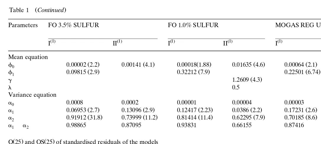
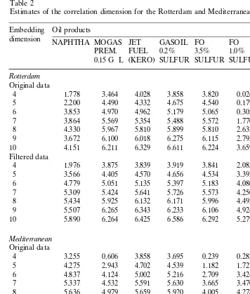
In the following tables we present our results. Table 2 contains the estimated correlation dimensions of the raw and filtered data for the Rotterdam and Mediterranean markets. By calculating the correlation dimension, one is able to decide whether a time series is generated by a dynamic process, with many or few degrees of freedom. In the case of many degrees of freedom, it is adequate to model the scalar time series by a stochastic process. In addition, by the correlation dimension it is possible to distinguish between periodic and chaotic dynamics, because a periodic dynamics results in an integer correlation dimension, whereas a chaotic results in a non-integer correlation dimension.
Starting with the correlation dimension, the first of the above criteria, we see from Table 2 that in five out of eight products of the Rotterdam market, namely
NAPHTHA, MOGAS PREM. 0.15 GrL, FO 3.5% SULFUR, FO 1.0% SULFUR
and MOGAS REG UNL, the estimated correlation dimension is lower than the embedding dimension and they satisfy the saturation condition. This can be an indication of a deterministic structure. Furthermore, the correlation dimension for these five oil products is consistent with Brock’s theorem, the second in the list of the above criteria. The estimates from the filtered data are not very different from the estimates from the raw data. In addition, the correlation dimension for the filtered data is slightly greater than that of raw data. Also, these five oil products
satisfy the Eckmann]Ruelle restriction, third in the list of the above criteria, as
Ž .
well. It seems, from Table 2 that in the case of JET FUELrKERO and MOGAS
PREM. UNL 95. the correlation dimension is lower than the embedding dimension and they satisfy Brock’s theorem but in these products it was observed that they do
not satisfy the Eckmann]Ruelle restriction.
To summarise, so far five out of eight oil products of the Rotterdam oil market satisfy the first three criteria in our list. Namely, they satisfy correlation dimension,
Table 2
a
Estimates of the correlation dimension for the Rotterdam and Mediterranean oil product markets Embedding Oil products
dimension NAPHTHA MOGAS JET GASOIL FO FO MOGAS MOGAS
PREM. FUELr 0.2% 3.5% 1.0% REG PREM.
Ž .
0.15 GrL KERO SULFUR SULFUR SULFUR UNL UNL 95 Rotterdam
Original data
4 1.778 3.464 4.028 3.858 3.820 0.026 3.417 3.993
5 2.200 4.490 4.332 4.675 4.540 0.179 4.417 4.580
6 3.853 4.970 4.962 5.179 5.065 0.305 4.924 5.195
7 3.864 5.569 5.354 5.488 5.572 1.770 5.212 5.711
8 4.330 5.967 5.810 5.899 5.810 2.633 5.680 5.810
9 3.672 6.100 6.018 6.275 6.115 2.795 5.692 6.242
10 4.151 6.211 6.329 6.611 6.224 3.659 6.016 6.577
Filtered data
4 1.976 3.875 3.839 3.919 3.841 2.085 3.787 3.962
5 3.566 4.405 4.570 4.656 4.534 3.392 4.480 4.626
6 4.779 5.051 5.135 5.397 5.183 4.080 5.012 5.215
7 5.309 5.424 5.641 5.726 5.573 4.250 5.538 5.581
8 5.434 5.925 6.132 6.171 5.996 4.495 6.056 6.000
9 5.507 6.265 6.343 6.233 6.106 4.924 6.043 6.261
10 5.890 6.264 6.425 6.586 6.292 5.279 6.052 6.587
Mediterranean Original data
4 3.255 0.606 3.858 3.695 0.239 0.282 NA NA
5 4.275 2.943 4.702 4.539 1.182 1.727 NA NA
6 4.837 4.124 5.002 5.216 2.709 3.424 NA NA
7 5.337 4.532 5.591 5.630 3.665 3.470 NA NA
8 5.636 4.979 5.659 5.920 4.005 4.278 NA NA
9 6.019 4.995 6.124 6.218 4.915 5.134 NA NA
10 5.972 5.085 6.463 6.301 5.169 5.122 NA NA
Filtered data
4 3.531 0.763 3.905 3.816 1.152 2.787 NA NA
5 4.337 2.988 4.578 4.530 1.473 3.609 NA NA
6 4.982 3.997 5.292 5.228 3.050 4.155 NA NA
7 5.553 4.473 5.770 5.676 3.704 4.491 NA NA
8 5.980 4.805 5.992 5.945 4.531 5.088 NA NA
9 6.129 5.235 6.300 6.278 4.820 5.829 NA NA
10 6.116 5.684 6.462 6.558 5.204 6.032 NA NA
a
NA, non-available.
found to satisfy the remaining two criteria in our list we will be in a position to argue that they are consistent with deterministic chaos. Regarding the other three products of the Rotterdam market with strong scepticism, it can be said that they are not consistent with deterministic chaos.
( )
E. Panas, V. NinnirEnergy Economics 22 2000 549]568 557
summarised as follows. On one hand the returns for NAPHTHA, MOGAS PREM.
0.15 GrL, FO 3.5% SULFUR and FO 1.0% SULFUR show the correlation
dimension to be lower than the embedding dimension, there is strong evidence for saturation of the estimated correlation dimension, the Brock’s theorem and the
Eckmann]Ruelle restriction are satisfied. On the other hand, the return series for
Ž .
GASOIL 0.2% SULFUR and JET FUELrKERO turn out to be more consistent
with a stochastic process. The empirical results for GASOIL 0.2% SULFUR and
Ž .
JET FUELrKERO are very instructive. One might naively conclude from Brock’s
theorem that the returns for both products demonstrate chaotic behaviour. This is
quite erroneous. Neither the Eckmann]Ruelle restriction nor the saturation
crite-rion is satisfied.
We now turn to a discussion of entropy index, K2. Recall that K2 entropy
measures the degree of chaos in a system. Table 3 represents the estimates of K2
entropy, for original as well as filtered data. Three striking conclusions emerge
Ž . Ž .
from Table 3: i K2 approaches saturation level except for the JET FUELrKERO
Ž .
and GASOIL 0.2% SULFUR for the Mediterranean and for JET FUELrKERO ,
GASOIL 0.2% SULFUR, MOGAS REG UNL and MOGAS PREM. UNL 95 for
Ž .
Rotterdam; ii K2-entropy estimates based on filtered data are greater than
Ž .
K2-entropy estimates based on the original data; and iii the K2-entropy results
also agree with the correlation dimension results. The correlation dimension
Ž .
results Table 2 and the convergence of the K2-entropy to a finite value for the oil
products NAPHTHA, MOGAS PREM. 0.15 GrL, FO 3.5% SULFUR, FO 1.0%
SULFUR and MOGAS REG UN provide a strong indication of chaotic behaviour for these products.
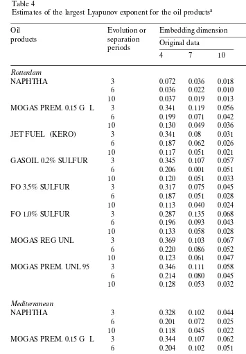
One of the most important characteristics of chaos is sensitivity to initial conditions. Lyapunov exponents measure the sensitivity of the system to changes in initial conditions, or determine the stability of the periodic orbits.
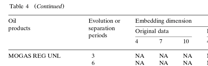
A positive value of the largest Lyapunov exponent is a characteristic of determin-istic chaotic behaviour and, in addition, provides a qualitative measure of the predictability of the system. Table 4 represent the largest Lyapunov exponents obtained using original and filtered data for both markets. The results of the above
Ž .
tables lead to the following conclusions: i in general, the largest Lyapunov exponents estimates are all positive, but differ according to the embedding dimen-sion, the evolution, and the original and filtered time series data used. This
Ž .
evidence strongly supports the presence of chaos in our returns series; ii If we
combine the results of correlation dimension, entropy, Eckmann]Ruelle condition,
and Brock’s theorem with the Lyapunov exponent estimates, the arising evidence
Ž .
supports that all products except for JET FUELrKERO and GASOIL 0.2%
Ž .
SULFUR for the Mediterranean and JET FUELrKERO , GASOIL 0.2%
SUL-FUR, MOGAS REG UNL and MOGAS PREM. UNL 95 for the Rotterdam are generated by a deterministic chaotic process. The results given in Table 4, there-fore, complement those given in Tables 2 and 3, which showed that the chaotic
behaviour for NAPHTHA, MOGAS PREM. 0.15 GrL, FO 3.5% SULFUR, FO
Ž .
Table 3
a
K2-entropy estimates for the oil products Embedding Oil products
dimension NAPHTHA MOGAS JET GASOIL FO FO MOGAS MOGAS
PREM. FUELr 0.2% 3.5% 1.0% REG PREM.
Ž .
0.15 GrL KERO SULFUR SULFUR SULFUR UNL UNL 95 Rotterdam
Original data
4 0.418 0.416 0.449 0.490 0.581 0.521 0.458 0.497
5 0.428 0.494 0.528 0.571 0.634 0.581 0.536 0.578
6 0.498 0.581 0.573 0.641 0.660 0.658 0.590 0.653
7 0.519 0.645 0.604 0.706 0.696 0.668 0.659 0.726
8 0.550 0.725 0.628 0.744 0.741 0.668 0.720 0.816
9 0.580 0.797 0.675 0.784 0.738 0.658 0.773 0.889
10 0.580 0.797 0.675 0.784 0.738 0.658 0.773 0.889
Filtered data
4 0.468 0.308 0.363 0.360 0.327 0.371 0.297 0.336
5 0.544 0.404 0.471 0.474 0.434 0.448 0.401 0.439
6 0.564 0.496 0.554 0.568 0.513 0.516 0.471 0.527
7 0.600 0.566 0.626 0.654 0.583 0.588 0.529 0.606
8 0.621 0.615 0.675 0.714 0.646 0.649 0.581 0.673
9 0.633 0.680 0.734 0.790 0.687 0.696 0.639 0.729
10 0.662 0.680 0.734 0.790 0.687 0.696 0.639 0.729
Mediterranean Original data
4 0.303 0.555 0.562 0.299 0.552 0.508 NA NA
5 0.390 0.630 0.639 0.371 0.630 0.592 NA NA
6 0.461 0.710 0.708 0.449 0.681 0.661 NA NA
7 0.510 0.748 0.773 0.508 0.698 0.667 NA NA
8 0.556 0.792 0.788 0.562 0.755 0.706 NA NA
9 0.596 0.870 0.855 0.612 0.842 0.704 NA NA
10 0.596 0.870 0.855 0.612 0.842 0.704 NA NA
Filtered data
4 0.304 0.563 0.335 0.370 0.501 0.423 NA NA
5 0.409 0.648 0.436 0.478 0.593 0.539 NA NA
6 0.496 0.732 0.530 0.576 0.659 0.635 NA NA
7 0.562 0.759 0.602 0.638 0.678 0.708 NA NA
8 0.619 0.793 0.669 0.716 0.724 0.763 NA NA
9 0.681 0.888 0.747 0.774 0.748 0.820 NA NA
10 0.681 0.888 0.759 0.774 0.748 0.820 NA NA
a
NA, non-available.
exponents characterise the horizon of prediction of the underlying model. That is, predictions based on periods longer than the order of the inverse of the largest Lyapunov exponent are not accurate. For example, the saturation value of the Lyapunov exponent in Table 4 in the case of FO 3.5% SULFUR is 0.066. Roughly,
Ž .
( )
E. Panas, V. NinnirEnergy Economics 22 2000 549]568 559
Table 4
a
Estimates of the largest Lyapunov exponent for the oil products
Oil Evolution or Embedding dimension
products separation Original data Filtered data
periods
4 7 10 4 7 10
Rotterdam
NAPHTHA 3 0.072 0.036 0.018 0.161 0.121 0.053
6 0.036 0.022 0.010 0.108 0.071 0.032
10 0.037 0.019 0.013 0.067 0.047 0.007
MOGAS PREM. 0.15 GrL 3 0.341 0.119 0.056 0.356 0.114 0.083
6 0.199 0.071 0.042 0.229 0.085 0.072
10 0.130 0.049 0.036 0.139 0.066 0.015
Ž .
JET FUELrKERO 3 0.341 0.08 0.031 0.384 0.131 0.105
6 0.187 0.062 0.026 0.217 0.108 0.090
10 0.117 0.051 0.021 0.137 0.071 0.079
GASOIL 0.2% SULFUR 3 0.345 0.107 0.057 0.396 0.214 0.140
6 0.206 0.001 0.051 0.227 0.163 0.138
10 0.120 0.051 0.033 0.132 0.120 0.104
FO 3.5% SULFUR 3 0.317 0.075 0.045 0.355 0.102 0.065
6 0.187 0.051 0.028 0.213 0.069 0.042
10 0.113 0.040 0.024 0.127 0.052 0.029
FO 1.0% SULFUR 3 0.287 0.135 0.068 0.352 0.140 0.074
6 0.196 0.093 0.043 0.253 0.101 0.045
10 0.133 0.058 0.028 0.139 0.053 0.042
MOGAS REG UNL 3 0.369 0.103 0.067 0.364 0.159 0.122
6 0.220 0.086 0.052 0.219 0.126 0.096
10 0.123 0.061 0.047 0.129 0.028 0.084
MOGAS PREM. UNL 95 3 0.346 0.111 0.058 0.351 0.124 0.101
6 0.214 0.080 0.045 0.218 0.101 0.074
10 0.128 0.053 0.032 0.141 0.065 0.067
Mediterranean
NAPHTHA 3 0.328 0.102 0.044 0.369 0.129 0.111
6 0.201 0.072 0.025 0.223 0.106 0.083
10 0.118 0.045 0.022 0.123 0.067 0.082
MOGAS PREM. 0.15 GrL 3 0.344 0.107 0.062 0.414 0.150 0.113
6 0.204 0.102 0.051 0.242 0.132 0.095
10 0.143 0.062 0.038 0.138 0.089 0.082
Ž .
JET FUELrKERO 3 0.333 0.082 0.034 0.366 0.112 0.072
6 0.205 0.057 0.025 0.217 0.089 0.063
10 0.122 0.043 0.024 0.131 0.059 0.059
GASOIL 0.2% SULFUR 3 0.339 0.105 0.050 0.379 0.248 0.152
6 0.212 0.089 0.055 0.240 0.190 0.149
10 0.122 0.058 0.039 0.154 0.116 0.116
FO 3.5% SULFUR 3 0.341 0.132 0.067 0.488 0.189 0.129
6 0.203 0.106 0.058 0.257 0.166 0.122
10 0.134 0.064 0.063 0.161 0.101 0.107
FO 1.0% SULFUR 3 0.339 0.113 0.056 0.384 0.133 0.095
6 0.217 0.079 0.045 0.225 0.109 0.078
Ž .
Table 4 Continued
Oil Evolution or Embedding dimension
products separation Original data Filtered data
periods
4 7 10 4 7 10
MOGAS REG UNL 3 NA NA NA NA NA NA
6 NA NA NA NA NA NA
10 NA NA NA NA NA NA
MOGAS PREM. UNL 95 3 NA NA NA NA NA NA
6 NA NA NA NA NA NA
10 NA NA NA NA NA NA
a
NA, non-available.
given oil product the values of the Lyapunov exponents decrease as the evolution length increases.
Ž
Before concluding this analysis, let us consider the BDS statistical test results in order to economise on space these results are available upon request from the
.
authors . They indicate that the time series returns are chaotic and not a stochastic process. We cannot rely upon BDS results, however, as our evidence indicates that the returns are non-linear processes with asymmetric distributions in all oil products. Therefore, the test is not appropriate in our case to provide a definite
Ž .
conclusion, see Hsieh 1991 .
3. Conclusions
We have reviewed and analysed several invariants for the empirical detection of chaotic structure for oil products in the Rotterdam and Mediterranean petroleum markets. The main empirical results obtained in the above analysis are summarised in Table 5.
They suggest that there is no variation among the markets concerning the chaotic behaviour of the data. The empirical and methodological-based results presented here indicate that:
v If explicit attention is not given to the construction of phase-space the
invari-ants may yield misleading results.
v In this paper, we pay careful attention to the construction of the phase-space,
which has important implications for the estimation of the various invariants. Thus, we would expect that errors in the estimates of invariants might be reduced by a better construction of phase-space.
v The empirical results of this paper suggest that particular care must be given to
( )
E. Panas, V. NinnirEnergy Economics 22 2000 549]568 561
Table 5
Summary of observed chaotic structures
Products Eckmann] Saturation Brock’s Entropy Saturation BDS Presence Ruelle correlation theorem Lyapounov statistic of
condition dimension exponent
Rotterdam
a
NAPHTHA Yes Yes Yes Yes Yes Non-ap. CHAOS
MOGAS PREM. 0.15 ? Yes Yes Yes Yes Non-ap. CHAOS
GrL JET FUELr No No Yes No No Non-ap. GARCH
ŽKERO.
GASOIL 0.2% SULFUR No No Yes No No Non-ap. GARCH
FO 3.5% SULFUR ? Yes Yes Yes Yes Non-ap. CHAOS
FO 1.0% SULFUR Yes Yes ? Yes Yes Non-ap. CHAOS
MOGAS REG UNL Yes Yes Yes Yes Yes Non-ap. CHAOS
MOGAS PREM. No No Yes No No Non-ap. GARCH
UNL 95
Mediterranean
NAPHTHA Yes Yes Yes Yes Yes Non-ap. CHAOS
MOGAS PREM. 0.15 Yes Yes Yes Yes Yes Non-ap. CHAOS
GrL JET FUELr No No Yes No No Non-ap. GARCH-M
ŽKERO.
GASOIL 0.2% SULFUR No No Yes No Yes Non-ap. CHAOS
FO 3.5% SULFUR Yes Yes Yes Yes Yes Non-ap. CHAOS
FO 1.0% SULFUR Yes Yes ? Yes Yes Non-ap. CHAOS
a
Non-ap., non-appropriate.
behaviour of time series. Frequently, the constraints are ignored or considered to be of secondary interest. In such cases, the correlation dimension, entropies, and Lyapunov exponents may produce poor or spurious results. Here, following
the Eckmann]Ruelle restriction, we cannot reach any definite conclusion from
our data for d2G6.1
Empirical analysis of identification of chaotic structure of return series
necessar-Ž
ily raises the question of filtering the transformation of the original data prior to
.
its analysis . The basic question underlying the estimates of various invariants is the adequacy of the data used to test the chaotic structure.
Comparisons of the invariants of the original and the residuals or GARCH filtered series in most cases tend to support Brock’s theorem.
However, the filtered data may give a false indication of chaos. In other words,
Ž Ž ..
filtering may affect the dimensionality of the original data see Chen 1993 and
the filtered data may mimic a chaotic one.
The above concludes the technical part of our analysis. It is good practice to make the connection between theory and practice. The present study focuses on oil markets and explores the possible non-linear price patterns.
The price series under study exhibit time varying volatility, excessive skewness, and kurtosis results, which suggest that price series contain non-linear dynamics. Methodologically ARCH-GARCH and chaos models are the non-linear models that are able to capture these symptoms. An ARCH-GARCH model is a stochastic process while a chaos model is a deterministic process.
The estimates of correlation dimension and Lyapunov exponents show that the commodities NAPHTHA, MOGAS PREM., SULFUR FO 3.5% and FO 1.0%, GASOIL and MOGAS REG. UNL. are chaotic time series. The correlation dimension gives an indication of the volatility of the given oil markets. Thus, correlation dimension can be a measure of the rate of information flow in the oil markets. On the other hand, Lyapunov exponents represent the rate at which the system creates or distorts information. For example in the case of NAPHTHA the correlation dimension is 5.972 and 4.151 in the Mediterranean and Rotterdam markets, respectively. This implies that for NAPHTHA the Mediterranean market
is 5.972r4.151s1.4 times more volatile than the Rotterdam market for the same
commodity. The estimates of Lyapunov exponents for NAPHTHA for both mar-kets are 0.022 and 0.013. If we consider a unit measuring error in the Mediter-ranean as well as in the Rotterdam market, then the error in the MediterMediter-ranean
market for NAPHTHA will be amplified 0.022r0.013s1.69 times faster than in
the Rotterdam market. In view of these findings, this study finds evidence of significant non-linear dependence in prices of these commodities. Thus, the
find-Ž .
ings of the present study are in agreement with the study by Savit 1989 , who concludes that self-regulating systems are generally characterised by a non-linear process. To the extent that oil markets are self-regulating systems with complex structures, the prices that these markets generate display non-linear chaotic process. In other words, for these commodities, the chaotic model suggests that there are several deterministic forces interacting with each other in such a way that complicated price movements can be produced in the Mediterranean and Rotter-dam oil markets. Given the information about the market structures, the future prices of the commodities are more likely to be subject to several deterministic
elements such as the influence of the Iran]Iraq and Iran]Kuwait conflicts, the
1991 international crisis in the Persian Gulf, and the changes in the OPEC pricing oligopoly.
In today’s world decisions are influenced by economic, environmental, and geopolitical factors. As a result, the complexity of all markets, including the oil markets, is very high. An energy economist who is interested in the dynamic behaviour of the complex system that governs the oil markets needs to know how sensitive the system is to initial conditions, and to achieve this he needs to estimate the Lyapunov exponents. An example that helps us clarify the above are the Iraqi
sales that began during a strong demand period } approximately 500 thousand
barrels per day}in December 1996. The reintroduction of Iraqi oil into the world
( )
E. Panas, V. NinnirEnergy Economics 22 2000 549]568 563
intense negotiations between the Iraqi government and the UN. It was, therefore, an exogenous shock of change in the initial conditions. This sudden change in the initial conditions will influence the dynamic behaviour of the time path of the oil prices.
Acknowledgements
The authors are grateful for the helpful comments and suggestions of an anonymous referee.
Appendix A: General methodology
A.1. Takens theorem or constructing a phase space
Let the price of oil product at time t be denoted by pt, then returns are
Ž .
measured as Ztslog ptrpty1 .
4
A scalar time series Zt, ts1,2,...,n represents observations, say from the
Rotterdam and Mediterranean markets, which usually have a multidimensional attractor. How can one study the original system by analysing the scalar signal
Zt4?
The key to modelling is that even if the exact description of the dynamic system under study is unknown, the state space can be reconstructed from a single scalar
Ž .
time series see Packard et al., 1980 . When the state space is reconstructed from a scalar time series it is usual to call this state space a phase space. The phase space is defined as the multidimensional space whose axes consist of variables of a dynamic system. An attractor can describe the asymptotic behaviour of the dy-namic system. The dimension of the attractor will provide a measure of the minimum number of independent variables that describe the dynamic system.
The state space reconstruction is the basis for recovering the properties of the original attractor from a scalar time series. Therefore, building a dynamic model from a scalar time series involves reconstructing a phase space from the data.
Ž .
A method of time delay coordinate has been suggested by Ruelle 1981 ; Takens
Ž1981 for this purpose. Takens 1981 showed that an attractor, which is topologi-. Ž .
cally equivalent to the scalar time series, can be reconstructed from a dynamic
system of n variables by using the time-delay coordinates. Specifically, given scalar
Ž . 4
time series Ztslog ptrpty1 , ts1,...,n the m dimensional signal Xt is
com-posed of the scalar series Zt as follows:
4 Ž .
Xts Zt,Ztqt,Ztq2t,...,ZtqŽmy1.t 6
Ž .
Thus, a point Xt in an m-dimensional phase space is defined by Eq. 6 and the
reconstructed variables provide qualitative information on the system dynamics. According to this procedure, the reconstruction of phase space simply consists of finding the embedding dimension and the time delay.
In the process of constructing a well-behaved phase space an important question
Ž . Ž .
is how to choose the time delay t and the embedding dimension m. Usually, the
procedure of determining the embedding dimension m is to increase m and to
estimate the fractal dimension or the largest Lyapunov exponent for every embed-ding dimension until the fractal dimension or the largest Lyapunov exponent remains almost constant. In almost all financial applications the value of the time
delay,t, determines the quality of the reconstructed trajectory in the phase space
and thus, the values obtained for the entropies.
The time delay, t, is usually chosen from the autocorrelation function of the
Ž
original time series see Tsonis and Elsner, 1988; Zeng et al., 1992; Tsonis et al.,
.
1993 . In this study, the time delay t is chosen such that the autocorrelation
Ž .
function attains the value of 1re see Zeng et al., 1992 .
A justification for the above procedure in the deterministic case is given by
Ž . Ž .
Takens’ theorem 1981 . As shown by Takens 1981 , the phase space retains the dynamic properties of the original state space, including the dimensionality. Main
Ž . Ž .
references include Takens 1981 , Sauer et al. 1991 .
According to Takens’ theorem, a condition for choosing the embedding
dimen-sion m is
Ž .
mG2Dq1 7
Ž .
where D is the attractor dimension in the sense of Hausdorff dimension . In
experimental practice, D is unknown. An estimate of the attractor dimension, D,
may be obtained from the correlation dimension.
A.2. The correlation dimension technique and Eckmann]Ruelle condition
In order to estimate the correlation dimension of the attractor, if it exists, from
4
the scalar time series Zt we follow the procedure described by Grassberger and
Ž .
Procaccia 1983 .
With this procedure the correlation dimension, a measure of phase space structure related to the fractal dimension, can be estimated from a scalar time series.
A correlation dimension, which provides the number of active degrees of freedom of the system, can be constructed in phase space as:
( )
E. Panas, V. NinnirEnergy Economics 22 2000 549]568 565
M
H u is Heaviside step function s
½
0 , if u-0
< <XiyXj< < is the norm computed between two vectors and MsnyŽmy1.t,
mŽ .
with n being the number of data points. The quantity C r for MªA is called
the correlation integral. When the system dynamics is governed by a strange
Ž .
attractor, it is possible to show see Grassberger and Procaccia, 1983 that for a
sufficiently small value of r
mŽ . DŽm. Ž .
C r ;r 10
Ž .
and that: limD m sd2.
mªA
Thus, if the value of d stabilises at some value dU, as the embedding dimension
2 2
increases, then dU is the estimated correlation dimension.
2
An important point, which has not been taken into account in financial time series applications, is the number of data points required for good estimation of the dimension of the attractor. The question of the length of the scalar time series
Ž
has been a major topic of debate see Wolf et al., 1985; Smith, 1988; Nerenberg
. Ž .
and Essex, 1990; Eckmann and Ruelle, 1992 . Eckmann and Ruelle 1992 suggest a minimal data length of
d2 U
r2 Ž .
n)10 11
A.3. Kolmogoro¨entropy
Correlation dimension is one of the techniques used in detecting the existence of chaos.
Ž .
This technique has some limitations, such as: i the need for a large amount of
Ž . Ž .
scalar time series data see Grassberger, 1986 ; and ii the influence of noise on its computation, which causes the correlation dimension to behave as if it were estimated from a stochastic time series; it was demonstrated by Osborne and
Ž . Ž .
Provenzale 1989 and Provenzale et al. 1991 that the detection of chaos based on
Ž .
the correlation dimensions by the Grassberger and Procaccia 1983 procedure can be spurious because of noisy systems with power-law spectra.
In addition, if the attractor has an integer correlation dimension, then it is not clear whether the process is chaotic. Thus, to detect the existence of chaos the correlation dimension should be complemented by other techniques, such as the
A useful quantity, which can be extracted from the correlation integral, is the
Ž .
KolmogorovK-entropy. Grassberger and Procaccia 1983 have proposed that
mŽ . Ž .
entropy estimate. The K2 entropy measures the degree of chaos in a system:
regular or ordered systems are characterised by K2s0, purely random systems by
Ž .
KªA, and chaotic deterministic systems by 0-K-qA.
A.4. Lyapuno¨exponents or sensiti¨e dependence on initial conditions
Lyapunov exponents give an additional feature that describes deterministic processes. These exponents measure the exponential divergence or convergence of nearby orbits. Points close together in phase-space are nearly identical states, points with separating orbits become unaligned with each other. The rate, at which such separation grows, expresses the extent to which the system’s dynamic behaviour is sensitive to small differences in initial states. The condition of sensitivity to initial conditions, which is characteristic of chaotic behaviour, implies exponential divergence of initially nearby orbits. Exponential divergence of the initially nearby orbits, measured by at least one positive Lyapunov exponent, serves
Ž .
to characterise a chaotic system quantitatively see Wolf et al., 1985 . There are n
Lyapunov exponents in a given n-dimensional system, but we need to estimate only
the largest one, namely lmax, which is defined by:
n
where « ti is the difference of infinitesimal neighbouring orbits on the attractor.
If the dimension of the attractor is not an integer, or if there is at least one positive Lyapunov exponent, the system is said to be chaotic. However, by applying only the largest positive Lyapunov exponent one cannot distinguish some non-linear models from chaotic models. In addition, the finiteness of the correlation and the information dimension as well as the largest positive Lyapunov exponent do not imply that one can definitely distinguish between a random process and a chaotic deterministic process. It should be recognised that these invariants are not statistical tests.
A.5. Brock’s residuals
Ž .
( )
E. Panas, V. NinnirEnergy Economics 22 2000 549]568 567
and the largest Lyapunov exponent of residuals from the best fitting time series model are the same as that of the original data.
A.6. BDS test
The limitation of Brock’s procedure is that no formal hypothesis testing is
Ž . Ž .
possible. However, Brock et al. 1986 proposed a stronger test the BDS test of the null hypothesis that a time series is generated by identically and independently
Ž .
distributed i.i.d. stochastic variables. The BDS test statistic is given by
m
1r2w mŽ . Ž 1Ž .. x Ž . Ž .
WsM C r y C r rsm r 14
mŽ . 1Ž . Ž . Ž .
where C r and C r are given in Eq. 8 and sm r is an estimate of the
standard deviation. Under the null hypothesis of an independent identical
distribu-Ž .
tion white noise , the W statistic converges as MªA to a standard normal
variable with mean zero and variance one. It was also demonstrated by Brock et al.
Ž1991 that the distribution of the. W statistic changes when applied on the
residuals ARCH and GARCH-type filters.
A large value of W is evidence of a non-linear model and a W value of 0
Ž .
indicates a stochastic process. Based on Monte Carlo results, Hsieh 1991 sug-gested that the BDS test statistic could detect other types of departures from i.i.d. such as non-linearity, non-stationarity and deterministic chaos. Therefore, rejection of i.i.d. does not imply chaos. In other words, the null hypothesis of i.i.d. may be rejected because of linear or non-linear dependence or chaotic structure. Finally,
Ž .
Hsieh 1991 suggested that the W statistic is not robust in detecting non-linear
processes with asymmetric distributions.
References
Blank, S.C., 1991. ‘Chaos’ in futures markets? A non-linear dynamical analysis. J. Future Markets 11, 711]728.
Bollerslev, T., Wooldridge, J.M., 1992. Quasi-maximum likelihood estimation of dynamic models with time varying covariances. Econom. Rev. 11, 143]172.
Brock, W.A., 1986. Distinguishing random and deterministic systems: abridged version. J. Econ. Theory 40, 168]195.
Brock, W.A., Dechert W., Scheinkman J., A Test for Independence Based on Correlation Dimension, unpublished manuscript, University of Wisconsin and Chicago, 1986.
Brock, W.A., Hsieh, D.A., LeBaron, B., 1991. Non-linear Dynamics, Chaos and Instability: Statistical Theory and Economic Evidence. The MIT Press, Cambridge, MA.
Chen, P., 1993. Searching for Economic chaos: a challenge to econometric practice and nonlinear tests.
Ž .
In: Day, R.H., Chen, P. Eds. , Nonlinear Dynamics and Evolutionary Economics. Oxford University Press, pp. 217]252.
DeCoster, G.P., Labys, W.C., Mitchell, D.W., 1992. Evidence of chaos in commodity futures prices. J. Future Markets 12, 291]305.
Fang, H., Lai, K., Lai, M., 1994. Fractal structure in currency futures price dynamics. J. Future Markets 14, 169]181.
Frank, M., Stengos, T., 1989. Measuring the strangeness of gold and silver rates of return. Rev. Econ. Stud. 56, 553]567.
Grassberger, P., 1986. Do climatic attractors exists? Nature 323, 609]612.
Grassberger, P., Procaccia, I., 1983. Measuring the strangeness of strange attractors. Physica 9D, 189]208.
Hsieh, D.A., 1991. Chaos and nonlinear dynamics: application to financial markets. J. Finance 46, 1839]1877.
Kohzadi, N., Boyd, M.K., 1995. Testing for chaos and nonlinear dynamics in cattle prices. Can. J. Agric. Econ. 43, 475]484.
Nerenberg, M.A.H., Essex, C., 1990. Correlation dimension and systematic geometric effects. Phys. Rev. A 42, 7065]7074.
Osborne, A.R., Provenzale, A., 1989. Finite correlation dimension for stochastic systems with power-law spectra. Physica D 35, 357]381.
Packard, N.H., Crutchfield, J.P., Farmer, J.D., Shaw, R.S., 1980. Geometry from a time series. Phys. Rev. Lett. 45, 712]716.
Provenzale, A., Osborne, A.R., Soj, R., 1991. Convergence of the K2 entropy for random noises with power-law spectra. Physica D 47, 361]372.
Ruelle D., 1981. Sensitive Dependence on Initial Conditions and Turbulent Behaviour. Bifurcation Theory and its Applications, Am. NY Academic Sci., New York, pp. 136]229.
Savit, B., 1989. Nonlinearity and chaotic effects in options prices. J. Future Markets 9, 507]518. Sauer, T., Yorke, J.A., Casdagli, M., 1991. Embedology. J. Stat. Phys. 65, 579]616.
Scheinkman, J.A., LeBaron, B., 1989a. Nonlinear dynamics and stock returns. J. Bus. 62, 311]337. Scheinkman, J.A., LeBaron, B., 1989b. Nonlinear dynamics and GNP data. In: Barnett, W., Greweke, J.,
Ž .
Shell, K. Eds. , Economic Complexity. Cambridge University Press.
Smith, L.A., 1988. Intrinsic limits on dimension calculations. Phys. Lett. A 133, 283]288.
Takens, F., 1981. Detecting Strange Attractors in Turbulence, Dynamical Systems and Turbulence in: Lecture Notes in Mathematics. Springer-Verlang, pp. 366]381.
Wolf, A., Swift, J., Swinney, H., Vastano, J., 1988. The weather attractor over very short timescales. Nature 333, 545]547.
Tsonis, A.A., Elsner, J.B., Georgakakos, K.P., 1993. Estimating the dimension of weather and climate attractors: important issues about the procedure and interpretation. J. Atmos. Sci. 50, 2549]2555. Wolf, A., Swift, J., Swinney, H., Vastano, J., 1985. Determining Lyapunov exponents from a time series,
vol. 16. Physica D, pp. 285]317.
Yang, S.R., Brorsen, B.W., 1993. Nonlinear dynamics of daily futures prices: conditional heteroskedas-ticity or chaos? J. Future Markets 13, 175]191.