Ruin probabilities based at claim instants for some non-Poisson
claim processes
q
David A. Stanford
a,∗, Krzysztof J. Stroi´nski
b, Karen Lee
aaThe Department of Statistical and Actuarial Sciences, Room WSC 211, The University of Western Ontario, London, Ont., Canada N6A 5B7 bThe University of Insurance and Banking, Warsaw, Poland
Received 2 October 1998; received in revised form 2 March 1999; accepted 3 May 1999
Abstract
The paper presents a recursive method of calculating ruin probabilities for non-Poisson claim processes, by looking at the surplus process embedded at claim instants. The developed method is exact. The processes considered have both claim sizes and the inter-claim revenue following selected phase type distributions. The numerical section contains figures derived from the exact approach, as well as a tabular example using the numerical approach of De Vylder and Goovaerts. The application of the method derived in the paper through numerical examples reveals the sensitivity of the value of probability of ruin to changes in claim number process. © 2000 Published by Elsevier Science B.V. All rights reserved.
JEL classifications: C690; C220
Keywords: Ruin probability; Recursive methods; Phase-type distributions; Non-Poisson risk processes
1. Introduction
This article is an extension of the results presented in Stanford and Stroi´nski (1994), dealing with the Sparre– Andersen risk process as defined, for instance, by Bowers et al. (1986). The process can be described as follows. The initial surplus isu, and premiums are earned at a constant rate. The inter-claim revenues (namely, the incomes received between successive claims) form a sequence of i.i.d. random variables (RVs) with a common distribution
A(x). Claim sizes are assumed to be non-negative i.i.d. RVs with a common distributionB(x).
The current extension to the earlier work considers the effect of some non-Poisson claim processes on the probability of ruin. The majority of previous work on ruin probabilities has assumed that claims occur according to a Poisson process. A notable departure is Asmussen et al. (1995) where other generalisations are referred to.
Since ruin occurs upon payment of claims, our approach here is to observe the surplus process embedded at claim instants only. We exploited this approach previously to obtain exact recursive formulae for the probability of ruin on
q
The graphs were prepared with the assistance of the late Lamia Abid. We are deeply moved and saddened by her untimely death, and she is remembered with great fondness. We dedicate this work to her memory.
∗Corresponding author. Tel.:+1-519-661-3612. E-mail address: [email protected] (D. A. Stanford)
a specified claim, in the case of a Poisson claim number process. Apart from being an exact method for calculating ruin probabilities, this approach has the advantage of revealing, in some sense, where the relative vulnerability to ruin lies over the duration of the process. In the limit, the recursive method produces ultimate probabilities of ruin, although other direct methods such as those of Asmussen (1992) and Asmussen and Rolski (1991) are better suited to that task. Finally, it is our hope that by concentrating on the risk process at claim instants, future research into related quantities such as the time and severity of ruin may benefit from insights gained from this new approach.
Caution has to be exercised when relating probabilities of ruin based at claim instants with classical finite-time ruin probabilities, as the former reflect in a different way the variation in the claim number process. There is no simple translation from the embedded probabilities to finite-time ruin probabilities, or vice versa. One might initially think of thenth claim instant as being a random quantity equal to the independent sum ofni.i.d. inter-claim times. However, ruin is more likely to occur if the inter-claim times are short, so the time of thenth claim and the likelihood of ruin on it are linked. Nonetheless, the embedded approach does afford an alternative view of the risk process.
Most efforts to date at determining the finite-time ruin probability (or its complement, the non-ruin probability) in the Poisson case can be classified into one of three groups. The solution to the integro-differential equation for the non-ruin probability (see Gerber (1979)) is typically stated in terms of Laplace transforms. Direct attempts at inverting the transform to obtain the probability of ruin have often encountered numerical difficulties (see, for instance, Janssen and Delfosse (1982) and Taylor (1978)). A second approach, followed by Garrido (1988) and others, is to employ diffusion approximations which retain the continuous-time aspect of the system under study and use an appropriate diffusion process to approximate the actual claims process. A third option, exploited by Dickson and Waters (1991) for instance, is to approximate the continuous-time process by one in discrete time.
The exact approach discussed here retains key aspects of both of these latter two approaches. The continuous-time process is retained, although ours is embedded at claim instants. In situations where it works in its entirety, there is no need to either discretise time or the claim size distribution. Thus questions on the accuracy of the discretisation and the size of the approximating discrete distribution are avoided. Similar to discrete time methods, integrals are replaced by recursive summations, however these are exact. Two of the three recursions for the coefficients in the predecessor to this paper involved only positive terms, with most if not all being between 0 and 1, and such recursions are known to be very accurate (see Grassmann (1990, p. 209)). It therefore is relevant to know how general a model can be accommodated to this approach, and conversely, what its limitations are.
The actual methodology consists of two parts: first, it is necessary to establish the basic recursion which indicates how the probability of ruin on thenth claim is related to the probability of ruin on the(n−1)th claim. This recursion involves expressions indicating the level of the surplus process on a specified claim number when ruin does not occur. Second, an algorithm entailing Laplace transforms is given, and mathematical induction is used to establish a particular form for the probability of ruin on thenth claim. In the current work we address two questions relating to the utility of the method for non-Poisson claim processes. First, we identify one type of non-Poisson behaviour where both steps of the methodology extend readily to provide a stable, exact algorithm for the probability of ruin. Secondly, in circumstances where the algorithm is complicated beyond a reasonable degree, we illustrate a discrete time approximation that can be adapted to the basic underlying recursion from the first step of the process.
An abbreviated development of the underlying theory is presented here. The interested reader is directed to Stanford and Stroi´nski (1994) for an expanded treatment. The introduction to that paper provided an overview of various methods for determining the probability of ruin, and the review paper by Taylor (1985) provides numerous references to work prior to that date. For developments since that time, we suggest the following papers which provide a flavour of the diversity of methods available: Gerber et al. (1987), De Vylder and Goovaerts (1988), Shiu (1988), Garrido (1988), Dickson and Waters (1991), and Asmussen and Rolski (1991).
2. Preliminaries
2.1. Phase-type distributions
Phase-type distributions have been used extensively in queueing theory and more recently in ruin theory to model continuous random variables (see, for instance, Asmussen and Rolski (1991)). The extensions to Stanford and Stroi´nski (1994) for the claim number process that we discuss in this paper belong to two subsets of phase-type dis-tributions that are popular for modelling purposes: the Erlang distribution and mixtures of exponential disdis-tributions. The phase-type formulation of these is presented below. Neuts (1981) provides a thorough treatment of phase-type distributions.
Essentially, the phase-type family includes all distributions which can be modelled as the time to absorption in a continuous-time Markov chain with a single absorbing state. The resulting distribution function for the time to absorption has the form
B(x)=1−γγγ ,exp(TTT x)eee, x ≥0,
whereγγγ is the row vector of probabilities of starting in the various transient states,eeea column vector of ones of appropriate size, andTTT is the matrix of transition rates among the various transient states. The corresponding density function isb(x)=γγγexp(TTT x)ttt0, x≥0, wherettt0= −TeTeTe. Its Laplace–Stieltjes transform (LST), which is denoted
by8B(s), is8B(s)=E{e−sX} =γγγ (sIII−TTT )−1ttt0.We consider below two well known subsets
2.1.1. Mixtures of exponentials
Such a mixture can be used as a simple model of distributions that are more variable than the exponential in terms of the squared coefficient of variation (denoted SCV), defined as SCV = Var[X]/(E[X])2. A mixture of exponentials has an SCV greater than or equal to 1. The phase-type formulation of a mixture ofMexponentials has the following form:
γ γ
γ=[r1, r2, . . . , rM], TTT = −diag[θ1, θ2, . . . , θM], ttt0=[θ1, θ2, . . . , θM]′,
b(x)= M X
i=1
riθie−θix, x≥0, E[X]= M X
i=1 ri
θi
, 8B(s)= M X
i=1 riθi
(θi+s)
.
We will use the mixture of exponentials to model inter-claim revenues that are more variable than the exponential.
2.1.2. Erlang-α
The Erlang-αdistribution is the subset of gamma distributions with integer-valued shape parameterα. It can be viewed as anα-fold convolution of the exponential distribution. It is often used as a simple model of distributions which are less variable than the exponential, since its SCV is given by 1/α. We will use it to model inter-claim revenues that are less variable than the exponential.
The phase-type representation of the Erlang-αcan be visualised as a movement throughαstates prior to absorption. Thus,
γγγ =[1,0, . . . ,0], TTT =
−θ θ 0
−θ θ
0 . .. −θ
, ttt0=
0
.. .
0
θ
.
Also,
b(x)= θ αxα−1 (α−1)!e
−θ x, x ≥0, E[X]=α/θ, 8 B(s)=
θ
θ+s
α
2.2. Notation and general formulae
We denote the distribution function of inter-claim revenue byA(y), its density function bya(y)and its LST by
8A(s)= Z ∞
0
e−sydA(y).
We defineB(y),b(y), and8B(s)as equivalent attributes of the claim size distribution. Letpn(y)be defined as
the incomplete density for the surplus after thenth claim. (It is of course incomplete because ruin may have already occurred. Integration ofpn(y)for all non-negativeyyields the probability of not being ruined by any of the firstn
claims.) Also, let the Laplace transform ofpn(y)be written as
Ln(s)= Z ∞
0
e−sypn(y)dy. (2.1)
Evaluating (2.1) ats=0 yields the probability of non-ruin up to thenth claim. Below, we develop a recursion between
Ln(s)andLn−1(s)which will enable us to determine the probability of ruin on thenth claim.
The increment between two consecutive claims is defined as the difference between the revenue earned and the subsequent claim amount. One can write the density function of the increment as
g(y)= ( R∞
0 a(y+t )b(t )dt, y≥0,
R∞
0 a(t )b(t−y)dt, y <0,
(2.2)
and its Laplace transform is
G(s)≡ Z ∞
−∞
e−syg(y)dy =8A(s)8B(−s). (2.3)
LetF (y)=R−∞y g(x)dxdenote the cumulative distribution function of the increment whose density function is defined by Eq. (2.2). The probability of ruin on the first claim isF (−u), that is the probability that the first increment is so negative that it uses up the whole initial reserve.
Our departure point for the current work is the recursive formula (2.7) from Stanford and Stroi´nski (1994), which is equally valid here
pn(y)= Z ∞
x=0
pn−1(x)g(y−x)dx, y≥0. (2.4)
In words, this convolution says that the level of the surplus at thenth claim instant, assuming that ruin does not occur, is the sum of the level at the(n−1)th claim instant plus the ensuing increment. When one takes Laplace transforms of (2.4) one obtains
Ln(s)=Ln−1(s)G(s)−
Z ∞
x=0
e−sxpn−1(x)
Z ∞
y=x
esyg(−y)dydx. (2.5)
Evaluating (2.5) ats=0, we find the probability of ruin on thenth claim is
P (n)≡Pr{ruin on the nth claim} = Z ∞
x=0
pn−1(x)
Z ∞
y=x
g(−y)dydx. (2.6)
3. Algebraic formulae for selected non-Poisson claims processes
In this section, two simple extensions of the Poisson claim number process are considered. The Poisson process has exponential inter-event times whose variance equals the square of the mean. The first extension we consider is the Erlang-αconsidered in Section 2 as an example of inter-claim times which are less variable than the exponential. The latter case considered is that of a mixture of exponentials, in order to consider a simple example of inter-claim times that are more variable than the exponential distribution. For the former, we will see that the methods of Stanford and Stroi´nski (1994) extend readily with a minor increase in complexity over the Poisson case. For the latter, we find that the extension becomes significantly more complicated even in its simplest case, although it is still tractable. In Section 4, we show that a pairing of our underlying recursion and the De Vylder–Goovaerts method can be used in these situations.
In each case considered, we first determine a difference equation involving the Laplace transformsLn(s), and then obtain an explicit expression forLn(s)via mathematical induction. Finally, corresponding expressions for the probability of ruin on thenth claim are found.
3.1. Recursions for Erlang-αinter-claim revenues
When the inter-claim revenue follows an Erlang-αdistribution and the claim sizes have a mixture ofNexponential distributions, a set of general formulae forLn(s)andP (n)can be determined as follows.
Theorem 3.1. For Erlang-αdistributed inter-claim revenue and a mixture ofNexponentials claim sizes,Ln(s), n≥
1,is given by
Proof. Under the stated assumptions
g(y)=
After substituting these expressions into (2.5) and after some manipulation one obtains the result (3.1).
Theorem 3.2. The general form ofLn(s), n≥1, when the inter-claim revenue distribution is Erlangian-α-distributed
and the claim sizes follow a mixture of two exponential distributions, is given by
and where the coefficientsc(n)j , Dm(n)andfj m(n), n≥2, satisfy the recursions
The coefficients are initialised as follows:
c(j1)=
Proof. The proof uses mathematical induction. Whenn =1, (3.1) already satisfies the general form ofLn(s)in
the theorem. We establish the remainder of the proof through the addition and subtraction ofA(ni −1)(λ/(λ+s))nα
to facilitate the factoring of the root(µi−s). In particular, we obtain
λ
After factoring the term(µi−s)from the first bracketed term of the last expression, and after reversing the order of
summation, it is readily seen that the coefficientscj(n)are related to the previous coefficients by (3.3). To complete the proof, we need to show that
A(n−1)(s)−Ai(n−1)=(µi−s)
After expanding this about indicesm=iandm=3−i, using (3.4), and employing the identity
k−n
isfj i(n) from (3.5). Therefore the final expression can be recognised as
A(n)(s), which completes the proof.
For exponential claim sizes we can state the following algorithm. We state this result without proof as the derivation is straightforward but tedious.
Ln(s)=e−uµ
In summary, the algorithms for the computation of the coefficientscj(n)in the case of Erlang-αrevenues are only slightly more complex than their Poisson counterparts. We note in particular that with the exception of the
A(n)(µi)term the algorithm consists of multiplications and additions of purely positive coefficients between 0 and
3.2. Recursions for mixtures of exponentially distributed inter-claim revenues
Theorem 3.3. For inter-claim revenue having a mixture ofMexponential distributions with weightsr1, . . . , rM
and ratesλ1, . . . , λM, and claim sizes having a phase-type distribution with representation (γγγ , TTT), wherettt0 =
−TeTeTe,Ln(s), n≥1, is given by
Ln(s)=
M X
i=1 ri
vvvi Z ∞
x=0
pn−1(x)exp(TTT x)dx−γγγ
λ
i
λi+s
Ln−1(s)
(sIII+TTT )−1ttt0, (3.7)
wherevvvi =λiγγγ (λiIII−TTT )−1.
Proof. For the stated inter-claim revenue and claim size distributions, the density of the increment becomes
g(y)=
PM
i=1riλie−λiy8B(λi), y ≥0,
PM
i=1riλiR0∞e−λitb(t−y)dt, y <0.
Substituting the expressions for phase-distributed claim sizes, and lettingvvvi =λiγγγ (λiIII−TTT )−1, the following is
obtained:
g(y)=
PM
i=1rivvvie−λiyttt0, y ≥0,
PM
i=1rivvviexp(−TTT y)ttt0, y <0.
(3.8)
Therefore
Z ∞
y=x
esyg(−y)dy= M X
i=1 rivvvi
Z ∞
y=x
esyexp(TTT y)dyttt0
= M X
i=1 rivvvi
Z ∞
y=x
exp((sIII+T)y)dyttt0= −esx
M X
i=1
rivvviexp(TTT x)(sI+TTT )−1ttt0. (3.9)
Substitution of (3.9) into the second term of (2.5) completes the proof. Evaluating (3.7) ats=0, and recalling Eq. (2.10) of Stanford and Stroi´nski (1994) one obtains the probability of ruin on thenth claim.
P (n)= M X
i=1 rivvvi
Z ∞
x=0
pn−1(x)exp(TTT x)dxeee. (3.10)
Theorem 3.4. The following general expressions forP (n)andLn(s)are obtained for mixtures ofMexponential
inter-claim revenues and Erlang-αclaim sizes:
P (n)= M X
i=1
α−1
X
k=0
riL(k)n−1(µ) (
(−µ)k k!
"
1−
µ
λi+µ
α−k#)
Ln(s)=
Proof. The proof is nearly identical to that presented in Section 2.3 of Stanford and Stroi´nski (1994), and is contained
in Lee et al. (1994).
Since (3.12) involves the term(µ/(µ−s))αit stands to reason that(µ−s)αmust be factored from the bracketed terms so that these factors will cancel when findingLn(s). Therefore we hypothesise the following general form
forLn(s)when claim sizes follow an Erlang-αdistribution:
Ln(s)=e−uµ
The proof of the correctness of this hypothesis whenα =1, together with the recursion for the coefficients, is given in the following theorem. (The interested reader is directed to Lee et al. (1994) for the derivations and proofs for a comparable form whenα=2. The same report includes numerical examples for bothα=1 andα=2.)
Theorem 3.5 (α=1: Exponential claim sizes). When the inter-claim revenue follows a mixture of two exponential
distributions, and for exponentially distributed claim sizes, the Laplace transform of the distribution of the reserve following the nth claim,Ln(s), n≥1, is given by (3.13) where the coefficientsc(n)j l at the nth stage are related to those at the(n−1)th stage by the following expressions forj =1,2, . . . , n:
where it is understood that sums of the formP-1
0(.)equal 0, and thatc
(n−1)
0l =0, for allland n. The algorithm is
initialised by settingc(101)=µ/(λ2+µ)andc(111)=µ/(λ1+µ).
Ln(s)=
After several changes of indices, and simplifying and cancelling the term(µ−s)one obtains
The proof is completed by collecting like terms and expressing the coefficients cj l(N ) as in (3.14) for
n=N.
Thus,P (n), n≥2 can be explicitly determined from (3.16) with coefficientscj l(n)starting fromc(101)=µ/(λ2+µ)
andc(111)=µ/(λ1+µ).
Numerical examples for this case are presented in Section 5. By inspection of Eqs. (3.13) and (3.14), we see that the recursion involves no negative numbers. Furthermore, the multiplications involve terms between 0 and 1, except for two combinatorial terms in the middle line. Thus, while the form of (3.14) may be complicated, it can nonetheless be programmed to provide accurate results.
Theorem 3.5 shows that the recursion for the coefficients, while tractable, is somewhat cumbersome. The situation is even more cumbersome forα=2. As an alternative to this exact method when the recursions are either too cum-bersome or intractable, an approximate method by De Vylder and Goovaerts can be adopted. This is presented next.
4. A numerical approach using the De Vylder–Goovaerts method
The methodology that we have employed to determine the ruin probability up to this point and in our previous paper consists of the following steps. First, a recursion involving the Laplace transforms of the incomplete densities
pn(x)is determined in terms of the density function for the incrementg(x). Next, an algebraic form forLn(s)is
obtained, and finally a recursion for the coefficients is developed. This procedure is tractable for the Poisson-arrival case, but can become an arduous task for certain arrival processes as we have seen in Section 3.2.
At the same time, it is possible to retain the advantages of working with the increment distribution and a recursion based at claim instants without having to determine explicit expressions forLn(s). Adopting the algorithm in De
Vylder and Goovaerts (1988, formulae (4) and (5)) we defineψn(u)=Pni=1P (i)to be the probability of ruin at or
before thenth claim, given the initial surplusu.
The probability of ruin on the first claim, as shown in Section 2, is obtained asψ1(u)=F (−u). The probability
that ruin occurs at or before thenth claim is obtained recursively as the sum of the probability that ruin occurs on the first claim, plus the complementary probability that a surplus(u+x) >0 resulted from the first incrementx, and the ruin occurs on or before the remaining(n−1)claims are paid. This yields
ψn(u)=F (−u)+ Z ∞
x=−u
g(x)ψn−1(u+x)dx. (4.1)
To obtain numerical results from the above formula (4.1) it was suggested by a referee to Lee et al.(1994) to discretise the density function of the increment and then to shorten the range of summation/integration by discarding small probabilities. The discretisation used will be based on formula (15) of De Vylder and Goovaerts (1988) rewritten as follows. Letfk,−∞< k <∞, be the probability mass function for the discretised increment distribution. Then
fk = Z k+1
x=k
F (x)dx− Z k
x=k−1
F (x)dx. (4.2)
One can obtain increasingly accurate discretisations by appropriate rescaling of the increment distribution. The formulae for the cumulative distribution function F (−u) are given below for the cases considered in Section 3.
Case 1. Mixture of exponentials revenue, Erlang-N claims
F (x)=
PM i=1qi
PN−1
n=0
λ
i
λi +θ
θ λi+θ
n
exθPNl=−0n−1(−xθ )
l
l!
, x <0,
PM i=1qi
"
1−
θ
λi +θ N
e−λix
#
, x ≥0.
Case 2. Erlang-Mrevenue, mixture of exponentials claims
Below we present the increment distribution for the following additional case:
Case 3. Mixture of exponentials revenue, mixture of exponentials claims
F (x)=
The determination of thefk’s for each case is straightforward. Below the final results for Case 3 are given:
F (−u)=
and the discretised increment distributionfk,−∞< k <∞, is given by
fk =
In the next section some numerical examples involving the exact method discussed in Section 3 are presented, as well as one example of the numerical approach discussed above.
5. Numerical results
In this section, selected numerical examples (Figs. 1–6) are presented to demonstrate the effects of the initial reserve ratio, relative security loading (RSL), and the variability of the inter-claim revenue (ICR) distribution (as measured by the SCV) on the probabilities of ruin.
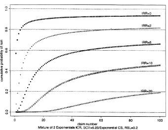
Fig. 1. Effect of initial reserve ratio (IRR).
Fig. 3. Effect of inter-claim revenue variability (SCV).
Fig. 5. Effect of relative security loading (RSL).
The initial reserve ratio (IRR) is defined as the initial reserve divided by the expected claim size, where the expected revenue between claims is given by
E[ICR]=(1+RSL)E[CS].
In the case of a mixture of two exponentials, the balanced means assumption(r1/θ1=r2/θ2=E[X]/2)is used
(see Stanford and Stroi´nski (1994, p. 248)).
Figs. 1–3 illustrate what happens when the ICR distribution is changed from exponential (corresponding to a Poisson claim arrival process) to a mixture of two exponentials. An exponential claim size is assumed in these examples. Fig. 1 illustrates how the probabilities of ruin decrease as the IRR increases. Here RSL=0.2 and the SCV of the ICR is 6.25. It is readily observed that when there is no initial reserve the probabilities of ruin are much higher than in the Poisson case. It is well known that the probability of eventual ruin for the Poisson claim number process when there is no initial reserve is 1/(1+RSL)(see Bowers et al. (1986 p. 359)). For example, under the Poisson case the probability of eventual ruin would be 5/6 when RSL=0.2. In contrast, the probability of ruin by the 20th claim for the mixture of exponentials with SCV=6.25 and the same RSL is already higher (see the highest curve on the graph). For IRR=0, it is obvious that the period of vulnerability starts immediately, while for IRR=20, it is notably delayed.
The effect of the RSL is explored in Fig. 2 when IRR=10 and SCV=6.25. As expected, as the RSL increases, the probabilities of ruin on individual claims decrease. For smaller values of RSL, the probabilities decay more slowly. One also notes that the curves reach their largest values sooner for larger RSL. If the RSL were large, for the same IRR, one would expect either to be ruined very soon or else a considerable reserve would be built up. Fig. 3 illustrates even more dramatically the effect of replacing the usual Poisson claim arrival process with a process that is more variable. Here, the various curves correspond to different values of the SCV. Note that the probabilities of ruin increase sharply as the SCV increases. This effect is somewhat moderated after the “peak” probabilities. The lowest probabilities of ruin on this figure correspond to the Poisson claim arrival process.
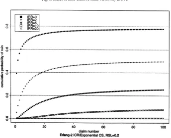
To complement the case of highly variable inter-claim times, Figs. 4–6 show what effect a more regular claim number process has on ruin than the usual Poisson claim number process. The ICR distribution in Figs. 4 and 5 is Erlang-2, whereas the CS distribution in all three figures is assumed to be exponential.
Fig. 4, like Fig. 1, explores the impact of the IRR when the RSL=0.2. If there is no initial reserve (the highest “curve” of probabilities in the graph), we can again compare with the previously determined ultimate probability of ruin for the Poisson case. It looks as though the cumulative probabilities of ruin stabilise and do not change much from, say, the 50th to the 100th claim. This probability is below 0.8 which is lower than the ultimate Poisson-case value of 5/6. The delayed onset of the period of relative vulnerability increases with the increase in IRR. However, even more visible from comparison of Figs. 1 and 4 is that the latter shows much reduced ruin probabilities due to the less variable claim arrival process. This difference is most pronounced for larger initial reserves.
Fig. 5 shows that the increase of the RSL both diminishes and shortens the period of vulnerability.
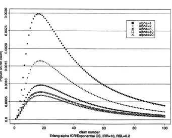
Fig. 6 explores the impact ofα on the ruin probability. It displays graphically the degree to which the ruin probability is reduced as the ICR variability (1/α) is decreased.
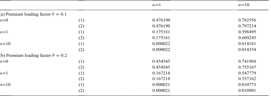
Table 1 presents a comparison of the exact probabilities of ruin obtained by using the algebraic approach with the corresponding values obtained from the numerical approach presented in Section 4. The layout of the table is adopted from Table 1 of Dickson and Waters (1991), and corresponds to a Poisson claims process with exponentially distributed claim amounts. The average claim size is 20, and relative security loadings of 10% and 20%, as well as initial reserve ratios of 0, 1, and 10 are considered. The discretised increment probabilities are likewise calculated until their sum exceeds 1−ǫ=1−10−6/3.
The key difference is that Dickson and Waters consider discrete time instants, whereas Table 1 here is calculated for claim numbers. This Poisson/exponential pairing also has the advantage of being able to apply a simpler algebraic form and the simplest expressions for the numerical recursions (4.8) and (4.9).
Table 1
A comparison of the algebraic (1), and the numerical (2) approaches
n=1 n=10
(a) Premium loading factorθ=0.1
u=0 (1) 0.476190 0.782556
(2) 0.476190 0.797214
u=1 (1) 0.175181 0.598495
(2) 0.175181 0.609245
u=10 (1) 0.000022 0.014181
(2) 0.000022 0.014354
(b) Premium loading factorθ=0.2
u=0 (1) 0.454545 0.741968
(2) 0.454545 0.755167
u=1 (1) 0.167218 0.547779
(2) 0.167218 0.557162
u=10 (1) 0.000021 0.010773
(2) 0.000021 0.010901
Determination of the numerical approach for the 100th claim was not possible from our PC-based Turbo Pascal programme, which encountered overflow errors.
Acknowledgements
This work has been financially supported by Canada’s Natural Sciences and Engineering Research Council through operating Grant No. OGP0041187 and through its summer scholarship programme. We wish to thank the referee, whose helpful comments have improved this paper.
References
Asmussen, S., 1992. Phase-type representations in random walk and queueing problems. The Annals of Probability 20, 772–789. Asmussen, S., Frey, A., Rolski, T., Schmidt, V., 1995. Does Markov-modulation increase the risk? ASTIN Bulletin 25, 49–66.
Asmussen, S., Rolski, T., 1991. Computational methods in risk theory: a matrix-algorithmic approach. Insurance: Mathematics and Economics 10, 259–274.
Bowers, N.L., Gerber, H.V., Hickman, J.C., Jones, D.A., Nesbitt, C.J., 1986. Actuarial Mathematics. Society of Actuaries, Itasca, Illinois. De Vylder, F., Goovaerts, M.J., 1988. Recursive calculations of finite-time ruin probabilities. Insurance: Mathematics and Economics 7, 1–8. Dickson, D.C.M., Waters, H.R., 1991. Recursive calculation of survival probabilities. ASTIN Bulletin 21, 199–221 .
Garrido, J., 1988. Diffusion premiums for claim severities subject to inflation. Insurance: Mathematics and Economics 7, 123–129.
Gerber, H.U., 1979. An Introduction to Mathematical Risk Theory. Monograph No. 8, S.S. Huebner Foundation, Distributed by R. Irwin, Homewood, IL.
Gerber, H.U., Goovaerts, M.J., Kaas, R., 1987. On the probability and severity of ruin. ASTIN Bulletin 17, 151–163.
Grassmann, W.K., 1990. Computational methods in probability theory. In: Heyman, D.P., Sobel, M.J. (Eds.), Handbooks in Operations Research and Management Science, Vol. 2, Stochastic Models, North-Holland, Amsterdam, pp. 199–254.
Janssen, J., Delfosse, P., 1982. Some numerical aspects in transient risk theory. ASTIN Bulletin 13, 99–113.
Lee, K., Stanford, D.A., Stroi´nski, K.J., 1994. Recursive methods for finite-time ruin probabilities for some non-Poisson Claim Processes. Technical Report TR-94-12. Dept. Statistical and Actuarial Sciences, The University of Western Ontario, London, Canada.
Neuts, M.F., 1981. Matrix-Geometric Solutions in Stochastic Models. John Hopkins University Press, Baltimore.
Shiu, E.S.W., 1988. Calculation of the probability of eventual ruin by Beekman’s convolution series. Insurance: Mathematics and Economics 7, 41–47.
Stanford, D.A., Stroi´nski, K.J., 1994. Recursive methods for computing finite-time ruin probabilities for phase distributed claim sizes. ASTIN Bulletin 24, 235–254.