Modelling of daily fluxes of water and carbon from
shortgrass steppes
Y. Nouvellon
a,∗, S. Rambal
b, D. Lo Seen
a, M.S. Moran
c, J.P. Lhomme
d,
A. Bégué
a, A.G. Chehbouni
e, Y. Kerr
f aCIRAD, 34093, Montpellier cedex 5, FrancebDREAM-CEFE, CNRS (UPR 9056) 34293, Montpellier cedex 5, France cUSDA-ARS, Phoenix, AZ, USA
dORSTOM/CICTUS, Hermosillo, Mexico eORSTOM/IMADES, Hermosillo, Mexico
fCESBIO-CNES, Toulouse, France
Received 27 October 1998; received in revised form 20 September 1999; accepted 5 October 1999
Abstract
A process-based model for semi-arid grassland ecosystems was developed. It is driven by standard daily meteorological data and simulates with a daily time step the seasonal course of root, aboveground green, and dead biomass. Water infiltration and redistribution in the soil, transpiration and evaporation are simulated in a coupled water budget submodel. The main plant processes are photosynthesis, allocation of assimilates between aboveground and belowground compartments, shoots and roots respiration and senescence, and litter fall. Structural parameters of the canopy such as fractional cover and LAI are also simulated. This model was validated in southwest Arizona on a semi-arid grassland site.
In spite of simplifications inherent to the process-based modelling approach, this model is useful for elucidating interac-tions between the shortgrass ecosystem and environmental variables, for interpreting H2O exchange measurements, and for
predicting the temporal variation of above- and belowground biomass and the ecosystem carbon budget. Published by Elsevier Science B.V.
Keywords: Simulation model; Water and carbon fluxes; Shortgrass ecosystem; Arid environment; SALSA program
1. Introduction
Arid and semi-arid rangelands constitute nearly one third of the earth’s land surface (Branson et al., 1972). The broad extent of arid and semi-arid regions and their sensitivity to climatic variations and land-use changes make it imperative to improve our
under-∗Corresponding author. Present address: USDA-ARS-USWCL,
SW Watershed Research Center, 2000 E. Allen Road, Tucson, AZ 85719, USA; Tel.:+1-520-670-6380; fax:+1-520-670-5550. E-mail address: [email protected] (Y. Nouvellon).
standing of the hydrologic, atmospheric and ecolog-ical interactions and sustainability of these systems. The Semi-Arid Land Surface Atmosphere (SALSA) program was conceived as a long-term, multidisci-plinary, monitoring and modelling effort to understand the complex interactions between hydrometeorolog-ical, biological and ecological processes occurring in semi-arid areas (Goodrich, 1994). The Upper San Pedro River Basin (USPB) was selected as the focal area for SALSA experiments. It spans the Mexico–US border from Sonora to Arizona and includes such major vegetation types as desert shrubsteppe, riparian
communities, grasslands, oak savannah and ponderosa pine woodlands. As part of the integrated SALSA objectives, research is focused on methods for esti-mating water, carbon and energy balance of semi-arid rangelands over large areas. One of the objectives is to develop coupled soil-vegetation-atmosphere (SVAT) and plant growth models that can assimilate remote sensing data (Goodrich et al., 1998) to scale up local results to the landscape or regional scale.
Such an approach requires that any plant growth model realistically describes temporal variability in the amount of live and dead aboveground biomass, Leaf Area Index (LAI), and percent cover. This in-formation is necessary to account for the influence of the vegetation canopy on the boundary layer (Lo Seen et al., 1997) and to couple with a land surface re-flectance model while performing the assimilation of remotely sensed data (Lo Seen et al., 1995; Mougin et al., 1995). In this paper, we present a process-based plant growth model for shortgrass ecosystems devel-oped in this perspective. The model has the same struc-ture as the model of Mougin et al. (1995) which had been developed and validated for annual grasslands of the Sahel. The main improvements needed were rel-ative to the presence of a root compartment whose dynamics cannot be ignored for perennial grassland ecosystems. These included allocation and transloca-tion processes between aboveground and belowground plant compartments. Also, a more physically-based description of the evapotranspiration process (based on Penman-Monteith (Monteith, 1965)) together with the aerodynamic and soil resistances have been included in the water budget submodel. The model retains the most important environmental variables affecting plant growth processes and operates with a daily time step using readily available daily meteorological data and a limited number of plant and soil parameters.
In the study region, plant growth and the determi-nation of peak biomass depend not only on highly unpredictable amounts of rainfall (Mc Mahon and Wagner, 1985), but also on carbohydrates previously stored in the root system. This storage pool is also a determining element in the response to grazing by large herbivores, in the survival during severe droughts, and in the domination of plant communities by perennial grass species. A realistic representation of belowground processes is therefore needed to suc-cessfully simulate aboveground growth patterns. The
model simulates the seasonal and inter-annual courses of aboveground live and standing dead biomass as well as leaf area of the dominant perennial grasses. The living root compartment permits inter-annual simulation of important processes such as transloca-tion of carbohydrates from roots to shoots during the early regrowth period at the end of the dry season and storage of photoassimilates in the belowground compartment. Also, as water is known to be the most important limiting factor on plant growth in semi-arid environments, soil water availability is computed in a water balance submodel. As in other published models (e.g. Feddes et al., 1978; Rambal and Cornet, 1982; Chen and Coughenour, 1994), plant growth and water fluxes processes are coupled in a functional and dynamic way.
While existing models account for more environ-mental effects on plant growth (e.g. Sauer, 1978; Detling et al., 1979; Coughenour et al., 1984; White, 1984; Hanson et al., 1988; Bachelet, 1989), some are difficult to parameterise (as stated in Hanson et al., 1985) or have been designed for other objectives. The model presented here retains only the most relevant processes so as to obtain a simplified yet realistic simulation. However, apart from simulating the one dimensional transfer of water and carbon, the model has some characteristics which makes it a candi-date for spatialization using remote sensing data. For example, it has kept to a minimum the number of spatially variable input parameters (meteorological driving variables and site specific parameters) and also simulates surface variables which can be used in reflectance or radiative transfer models.
Here, this paper only gives a description of the model together with its validation on a grassland site of the USPB during three consecutive growing sea-sons. How the model is used in a scheme for including remote sensing data is not described at this stage, as this is the subject of ongoing work.
2. Model description
2.1. General model structure
The main processes involved in the plant growth sub-model are photosynthesis, allocation of photosynthates to shoots and roots, translocation of carbohydrates from roots to shoots during the early growing pe-riod at the beginning of the wet season, respiration, and senescence. Many physiological processes such as photosynthesis and senescence are dependent on water availability in the root zone, which is simulated in a water balance submodel.
2.2. Vegetation growth model
The time course of biomass in the compartments is described by three differential equations with respect to time (t):
biomass, living root biomass and standing dead biomass, respectively; Pg is the daily gross
photo-synthesis; aa and ar are the photosynthate allocation
partition coefficients to shoot and root compartments (aa+ar=1); Tra represents the translocation of
car-bohydrates from the roots to the living aboveground compartment; Rat and Rrt are total daily amounts of
respiration from aboveground and root compartments,
Sa and Srrepresent the losses of biomass of the living
shoots and roots due to senescence; and L represents the litter fall. Bag, Br, and Bad, are expressed in g
DM m−2.
2.2.1. Photosynthesis
The daily carbon increment for the whole system results from photosynthesis. The gross daily canopy photosynthesis can be expressed as
Pg=SεcεIεbf1(9l)f2(T ) (4)
where S is the daily incoming solar radiation;εc the
climatic efficiency (Photosynthetically Active Radi-ation (PAR)/S); εI the efficiency of interception by
green leaves (or f PAR=intercepted PAR/PAR); and
εb is the energy conversion efficiency (or g
assimi-lated CH2O per unit of intercepted PAR). Functions
f1and f2 account for the constraints imposed by
wa-ter stress, leaf wawa-ter potential,9l, and temperature, T
respectively.
Water stress reduces photosynthesis by limiting the CO2 diffusion from air to leaf tissues as a result of
stomatal closure. It is expressed as a function of leaf water potential as in Rambal and Cornet (1982):
f1(9l)=
(1.64rs min+rm+1.39ra)
(1.64rsc+rm+1.39ra) (5)
where rsc and rs minare current and minimum canopy
stomatal resistance to water vapour; and rmand raare
mesophyll resistance and canopy boundary layer re-sistance to water vapour. The constants 1.64 and 1.39 relate to the ratio of diffusivities of CO2 and water
vapour in the air at 20◦C, and the ratio of the rate of transfer of CO2and water vapour in the canopy
bound-ary layer, respectively. rsc is calculated as a function
of9l(see below). For C4grasses, rmis approximately
80 sm−1 (Gifford and Musgrave, 1973; Jones, 1992), and rs min100 sm−1(Rambal and Cornet, 1982).
To calculate f2, we assume a null daily
photosyn-thesis for temperatures smaller than a minimum tem-perature, and a linear relationship between photosyn-thesis and daily mean air temperature for temperatures ranging between minimum and optimum temperature.
f2(T) can be expressed by:
where Tmin and Topt are the minimum and optimum
temperature for gross photosynthesis of C4 grasses,
respectively 7◦C (Sauer, 1978) and 38◦C (Penning de
Vries and Djitèye, 1982).
The climatic efficiencyεcis fixed to 0.47 (Szeicz,
1974), and the interception efficiencyεIis calculated
Ld=SdBad (9) Lt =Lg+Ld (10)
where Ld is the dead biomass LAI; Sgand Sd are the
specific leaf areas of the aboveground green biomass and the standing dead biomass [0.0105 m2g−1 and
0.0110 m2g−1, respectively (Goff, 1985)]; k
1has been
measured in a similar semi-arid grassland to be 0.58 (Nouvellon, 1999).
The energy conversion efficiencyεbis dependent on
the physiological age and therefore varies during the growing season. The depressing effect of leaf aging onεbis taken into account:
εb=εb maxf3(age) (11)
whereεb max is the maximum energy conversion
effi-ciency for young mature tissues, and f3is an empirical
function representing the effect of aging onεb. The
physiological leaf age and f3were calculated as in the
BLUEGRAMA model (Detling et al., 1979).εb maxis
usually taken as 8 g DM MJ−1 (Charles-Edwards et al., 1986).
2.2.2. Allocation
The available carbon pool resulting from photosyn-thesis is allocated into above-and belowground parts according to the allocation coefficients, aa and ar,
re-spectively. The daily amount which should be translo-cated from shoot to root Taris calculated according to
Hanson et al. (1988). Their model is based on the as-sumption that a balance must be maintained between shoots and roots such that the amount of aboveground phytomass that the present root biomass can support is not exceeded. The excess amount of biomass in the shoots is determined as:
Bax=rxBag−Br (12)
where rxis the root to shoot ratio below which
translo-cation occurs, set to 10 for perennial warm season grass (Hanson et al., 1988). If Bax> 0, biomass flows
from the shoots to the roots. If not, there is no alloca-tion. Taris calculated so that the root to shoot ratio is
fixed to rxon a daily basis: rx= Br+Tar
Bag−Tar
(13)
which, when combined with Eq. (12), means that:
Tar= Bax
1+rx
(14)
Allocation coefficients are calculated assuming that
Tarshould not exceed the gross photosynthesis Pg: ar=
Tar/Pg
1
ifTar< Pg
ifTar≥Pg (15)
The allocation coefficient for aboveground parts is cal-culated as:
aa=1−ar (16)
When the calculated shoot senescence exceeds a crit-ical rate of 0.012, ar is given a value of 0.71. This
value is based on results of Singh and Coleman (1975) who found that during the late growth stage of the semi-arid shortgrass blue grama (Bouteloua gracilis (H.B.K.) Lag.), 71% of the photoassimilated radiocar-bon moved to roots.
2.2.3. Root to shoot translocation
Translocation of carbohydrates from roots to shoots,
Tra occurs during the early season regrowth or later
in the season if some process such as grazing has re-moved a critical amount of green biomass. The model used to calculate Trais the one proposed by Hanson et
al. (1988), which necessitates three conditions for this process to occur: (1) The average 10 day soil tempera-ture must be greater than 12.5◦C; (2) the average 5 day soil water potential must be greater than −1.2 MPa, and; (3) Br> rxBag.
If all these conditions are met:
Tra=trBr (17)
where tris the proportion of root biomass translocated
daily to shoots (=0.005 at 25◦C). We assume that translocation is temperature dependent with a Q10=3.
2.2.4. Respiration
Total respiration Rtis the sum of total aboveground
respiration, Rat,and total root respiration, Rrt. For C4
grasses photorespiration is negligible. Thus, the above-ground respiration Ratcan be expressed as the sum of
maintenance and growth respiration:
and the total root respiration Rrtis expressed as: Rrt =mrf4(T )Br+gr(arPg) (19)
where ma and mr are the maintenance respiration
coefficients for aboveground and root biomass; f4(T)
represents the effect of temperature on maintenance respiration (Q10=2); ga and gr are the growth
res-piration coefficients for aboveground and root com-partment, respectively. These coefficients represent the cost for producing new biomass (McCree, 1970; Amthor, 1984). ga and gr are approximately 0.25
(McCree, 1970; Penning de Vries and Djitèye, 1982; Amthor, 1984; Ruimy et al., 1996) and 0.2 (Bachelet, 1989), respectively. Shoot maintenance respiration is 0.02 g DM per g DM per day at 20◦C (Amthor,
1984). Root maintenance respiration is 0.002 g C (g metabolic C day)−1 (Bachelet, 1989) at 20◦C.
As-suming 60% of structural material in roots (Bachelet, 1989), this led to an overall maintenance respiration rate of 0.0008 g DM per g DM per day.
2.2.5. Senescence
The amounts of green aboveground biomass and root biomass which die each day, Sa and Sr, are
cal-culated as:
Sa=daBag (20) Sr=drBr (21)
where da and dr are the death rate for aboveground
part and roots, respectively. dais calculated as a
func-tion of leaf physiological age, plant water potential and daily minimum temperature according to Detling et al. (1979). davaries from 0.0074 for young well-watered
shoots, up to 0.14 for old shoots at −5 MPa. These values are close to those used by Coughenour et al. (1984) and Bachelet (1989). dr is assumed to be
con-stant during the year, and was calculated based on the results of Anway et al. (1972) who estimated the root biomass replacement rate of blue grama as 25% per year.
2.2.6. Litterfall
Transfer of material from standing dead biomass to litter can be caused by wind, rain and dust (Clark and Paul, 1970). We assumed that the effects of dust and wind were negligible compared to the effect of rain.
The rate of standing dead biomass pushed down by rain on a given day (kr) was calculated as in Hanson
et al. (1988):
kr=0.25 [1−exp(−0.025R)] (22)
where R is the total daily precipitation (in mm), and −0.025 is the tolerance of standing dead biomass to precipitation for warm season grass (Hanson et al., 1988). Daily litter production (La) is thus:
La=krBad (23)
2.3. Water balance model
The water balance model follows the general scheme described in Leenhardt et al. (1995). It uses a simplified two layer canopy evapotranspiration model coupled with a multilayered soil water balance. A top 0–0.02 m soil layer controls the direct evaporation and two deeper layers (0.02–0.15 and 0.15–0.60 m) participate in both evaporation and plant water uptake.
2.3.1. Soil water balance
Each soil layer is characterised by its water content
θ and water potential ψ; these two variables are re-lated by the widely used power-function model for the retention curve first proposed by Brooks and Corey (1964) and further simplified by Campbell (1974) and Saxton et al. (1986):
ψ=Aθb (24)
Changes in soil water content are simulated by a mul-tilayered bucket model with a daily time step. The water infiltrating the soil is distributed down the pro-file according to the bucket model: the soil layers are filled successively from top to bottom untilθ reaches field capacity. We assumed that field capacity is equal to the water content at−33 kPa soil water potential. The daily change of the soil water content of the first layer of depth z1is:
1θ1=
R−Es1−D1
z1 (25)
where R is the amount of rainfall (mm), D1 the
drainage from the first layer to the second (mm); and
Es1 is the evaporation from the first layer (mm). In
1θi =
Di−1−Esi−Qci−Di zi−zi−1
(26)
where i is the soil layer number; Di−1 the water
in-filtrated from the previous layer (mm); and Qci is the
water extracted from the layer i for transpiration (see next section) (mm). Drainage from a layer i to layer
i+1 occurs whenθi>θfci, whereθfci is the field
ca-pacity (mm3mm−3).
2.3.2. Estimation of actual evapotranspiration
The total evaporation from the sparse discontinu-ous grass canopy is calculated as the sum of bare soil evaporation Esand canopy evaporation EC. ECand Es
are calculated empirically from the evapotranspiration of a continuous canopy and evaporation of a bare soil regardless of their percentage covers. If fvg, fvd and
fs are respectively, the cover fraction of green
vegeta-tion, dead vegetation and bare soil (fvg+fvd+fs=1),
Ec and Es are calculated based on Penman-Monteith
equation (Monteith, 1965) as:
Ec=fvg
where A is the available energy, which is the difference between net radiation Rn and soil heat flux G; D the
vapour pressure deficit of the air at a reference height above the surface;λthe latent heat of vaporisation;ρ
air density; cpthe specific heat of air at constant
pres-sure;γthe psychrometric constant and s is the slope of the saturated vapour pressure curve at the temperature of the air Ta; rscand rssare the surface resistances for
a full canopy and a bare soil, respectively; and racand
rasare the corresponding aerodynamic resistances. fvg
and fvd are calculated as a function of Lgand Ld:
The evaporation Esis distributed between the different
layers of the soil profile following an extinction coef-ficient which depends on soil water content, thickness and depth of each layer (Van Keulen, 1975; Rambal and Cornet, 1982).
In the model, rainfall interception by the canopy, and the subsequent evaporation of intercepted wa-ter are not considered. In shortgrass ecosystems, the amount of water intercepted by the canopy is usu-ally limited by low aboveground biomass and percent cover, but it may not be negligible during the growing season if several rainfall events occur during the day (Thurow et al., 1987; Dunkerley and Booth, 1999). It was assumed that evaporation of intercepted water is compensated by an equivalent reduction in transpira-tion, so that it does not increase total evapotranspira-tion.
2.3.3. Estimation of available energy
The available energy A is the difference between net radiation Rn and soil heat flux G. Rn and G are
estimated as follows:
Rn=Sn+Ln (31)
where Snis the net short-wave radiation; and Lnis the
net long-wave radiation. Snis given by:
Sn=S(1−α) (32)
where S is the incoming short-wave radiation; andαis the albedo of the surface (taken to be equal to 0.3 for a bare soil and 0.2 for dense canopy). Lnis calculated
with a Brunt-type equation (Shuttleworth, 1993).
Ln= −c(ae+be√e)σ (Ta+273.2)4 (33) where c is an adjustment coefficient for cloud cover; e is the vapour pressure in KPa; aeand beare regression
coefficients (=0.34 and−0.14, respectively);σ is the Stefan-Boltzmann constant; and Ta is the mean air
temperature in ◦C. The coefficient of adjustment for cloud cover is given by:
c=ac
S
So
+bc (34)
where Sois the solar radiation for clear skies,
calcu-lated as a function of day of year and latitude following Perrin de Brichambaut and Vauge (1982); ac=1.35
and bc= −0.35 for arid areas (Shuttleworth, 1993).
For a bare soil from which water can evaporate dur-ing the whole day, Lnis calculated over 24 h and G is
equal to 5% of (Sn+Ln), and Lnis calculated over the
daylength.
2.3.4. Resistance models
The bulk stomatal resistance of the canopy rscis
cal-culated as a function of leaf water potential9l(MPa)
as:
where rs min is the minimal stomatal resistance
ob-served in optimal conditions; 91/2 the leaf water
potential corresponding to a 50% stomatal closure (MPa); and n is an empirical parameter (Rambal and Cornet, 1982).
The soil surface resistance rss is calculated as a
function of the water content of the first soil layer by means of an empirical relationship (Camillo and Gurney, 1986):
rss=4140(θs1−θ1)−805, (s m−1) (36)
whereθ1represents the water content of the top soil
0–0.02 m layer (m3H2O m−3soil);θs1is the soil water
content at saturation (m3m−3) of the ground surface layer.
The aerodynamic resistances are calculated as:
ra= ln 2[(z
r−d)/z0]
(k2U ) (37)
where zr is the reference height where wind speed
U and air humidity are measured; k the von Karman
constant (0.41); d the zero plane displacement; and
z0is the roughness length calculated as a fraction of
the mean height hcof the vegetation canopy, z0=0.1
hc and d=0.67 hc. For a bare soil, z0=0.01 m and
d=0. hc is approximately 0.12 m for this shortgrass
ecosystem (Goff, 1985; Weltz et al., 1994).
2.3.5. Calculation of leaf water potential
The leaf water potential9lis needed to calculate the
canopy resistance and hence the canopy transpiration. It is obtained iteratively by equating Ec[given by Eq.
(27) in which rsc is replaced by its formulation in Eq.
(35)] with the sum of the water amounts extracted by the roots from the different soil layers, as calculated following an analogy with Ohm’s law:
Qi=
(9si−9l) rspi
(38)
where rspiand9siare the soil-plant resistance and the
water potential in the ith soil layer. At the daily time scale used in the model, we assume that internally stored water does not contribute significantly to tran-spiration and that the canopy generates a water poten-tial just sufficient to equal transpiration and root wa-ter uptake (Rambal and Cornet, 1982). At lower time scale, models have been proposed to account for the variation of water storage in the canopy (Kowalik and Turner, 1983). rspiis a linear function of root biomass
in the ith layer, and9si is inferred from θi through the soil retention curve9s=f(θ).9l of day n is
cal-culated from9siof day n−1, and is used to calculate
rsc and Ec of day n.
3. Calibrating and testing the model
3.1. Site description and experimental setup
average frost-free season is 239 days. Relative humidity is low throughout the year (average value=39.5%). April–June have the lowest relative humidity and August and September the highest. During December and January, high values are also common due to effects of frontal rain events. The mean annual wind speed is about 3.6 m s−1.
The vegetation cover within the Kendall study area is dominated by C4perennial grasses whose dominant
species are black grama (Bouteloua eriopoda (Torr.) Torr.), curly mesquite (Hilaria belangeri (Steud.) Nash), hairy grama (Bouteloua hirsuta (Lag.) and three-awn (Aristida hamulosa (Henr.)) (Weltz et al., 1994), and whose root systems are almost exclusively restricted to the upper 60 cm of soil (Cox et al., 1986; Nouvellon, 1999).
Rainfall was monitored at the Kendall site, using automated weighing raingauges (Renard et al., 1993). Other ancillary meteorological data included wind speed, measured at 2 m Above Ground Level (AGL) using a R. M. Young photo-chopper cup anemometer, solar radiation, measured at 3.5 m AGL using a LiCor silicon pyranometer model LI-200SZ, and relative air humidity and air temperature, measured at 2 m AGL using a Campbell Scientific Inc. (CSI) temperature and relative humidity sensor model 207 contained in a Gill radiation shield (Kustas and Goodrich, 1994; Kustas et al., 1994). Net radiation was also measured, at 3.3 m AGL with a REBS Q*6 net radiometer (Kus-tas et al., 1994; Stannard et al., 1994), as well as soil moisture from Time Domain Reflectimetry (TDR) probes spaced every 0.1 m down to a depth of 0.6 m (Amer et al., 1994).
Biomass and LAI were estimated at the Kendall site at 2 weeks to 1 month intervals during the grow-ing seasons, and approximately at 1.5 month intervals between the growth periods (Tiscareno-Lopez, 1994). Each estimation of live and dead standing biomass re-sulted from clipping plants within eight 0.5 m×1.0 m quadrats, and weighing them after a 24 h drying period at 70◦C.
3.2. Model parameters
A number of attempts have been made to predict retention curves from soil texture data (e.g. Arya and Paris, 1981; Rawls et al., 1982; De Jong, 1983 and
Saxton et al., 1986). These attempts have not been completely successful (e.g. Ahuja et al., 1985). Nev-ertheless, the relationship between soil water content and soil water potential is strongly dependent on soil texture. In this study, we assume the broad-based re-gression equations proposed by Saxton et al. (1986) which adequately predict the two parameters of the moisture retention curves (Eq. (24)) as a function of measured soil particle size distribution in each soil layer. For the 0.02–0.15 and 0.15–0.60 m soil layers the b parameters calculated following this regression and measured soil textures are−8.71 and−8.51, re-spectively. These values are rather low compared to that obtained by Clapp and Hornberger (1978) from the statistics of moisture parameters for sandy clay loam soils (−7.12±2.43).
Parameters describing root biomass distribution were set following the results of Cox et al. (1986) who measured root biomass distribution on a similar semi-arid grassland close to this site in August 1983. According to their results, 73% of root biomass was found in the first 0.15 m. These results were close to those of Singh and Coleman (1975) who found on a shortgrass prairie, dominated by blue grama, that 68–78% of the total root biomass occurred be-tween 0 and 0.20 m. Other model parameter values are summarised in Table 1.
Initial water content in the soil layers, as well as dead and living aboveground biomass were measured. Initial root biomass was fitted so that simulated above-ground biomass compared well with the first measure-ments of the 1990 growing season. As expected, this value (444 g DM m−2) was close to but less than the value obtained at a later stage during the 1983 grow-ing season (Cox et al., 1986).
3.3. Simulation results
compar-Table 1
List of parameters used in the model
Parameters Symbol Equation Value Unit Reference
Climatic efficiency εc Eq. (4) 0.47 Szeicz, 1974
Minimum canopy stomatal resistance
rsmin Eq. (5) 100 sm−1 Rambal and Cornet,
1982
Mesophyll resistance rm Eq. (5) 80 sm−1 Gifford and Musgrave,
1973; Jones, 1992 Minimum temperature
for gross photosynthesis
Tmin Eq. (6) 7.0 ◦C Sauer, 1978
Optimum temperature for gross photosynthesis
Topt Eq. (6) 38.0 ◦C Penning de Vries and
Djit`eye, 1982 Extinction coefficient of
radiation in the canopy
k1 Eq. (7) 0.58 Nouvellon, 1999
Specific leaf areas of the aerial green biomass Sg
Sg Eq. (8) 0.0105 m2g−1 Goff, 1985 (measured
on Kendall site) Specific leaf areas of the
aerial dead biomass Sd
Sd Eq. (9) 0.0110 m2g−1 Goff, 1985 (Measured
on Kendall site) Maximum energy
conversion efficiency
εbmax Eq. (11) 8 g DM MJ−1 Charles-Edwards et al., 1986 Minimum root to shoot
ratio
rx Eq. (12) 10.0 Hanson et al., 1988
Proportion of root biomass daily translo-cated to shoots
tr Eq. (17) 0.005 Hanson et al., 1988
Maintenance respiration coefficient for aerial biomass
ma Eq. (18) 0.02 (at 20◦C) g DM per g DM per day
Amthor, 1984
Maintenance respiration coefficient for root biomass
mr Eq. (18) 0.0008 (at 20◦C) g DM per g DM
per day
see text
Growth respiration coef-ficient for aerial biomass
ga Eq. (18) 0.25 McCree, 1970
Growth respiration coef-ficient for root biomass
gr Eq. (18) 0.2 Bachelet, 1989
Death rate for aerial compartment
da Eq. (20) 0.0074 to 0.14 g DM per g DM per day
Detling et al., 1979 Death rate for root
compartment
dr Eq. (21) 0.00078 g DM per g DM
per day
see text and Nouvellon, 1999 Extinction coefficient of
radiation coming from zenith in the canopy
k2 Eqs. (29) and (30) 0.36 Nouvellon, 1999
Albedo α Eq. (32) 0.3 (soil) 0.2 (canopy)
Leaf water potential cor-responding to a 50% stomatal closure
91/2 Eq. (35) 0.6 MPa Rambal and Cornet, 1982
Shape parameter n Eq. (35) 5 Rambal and Cornet, 1982
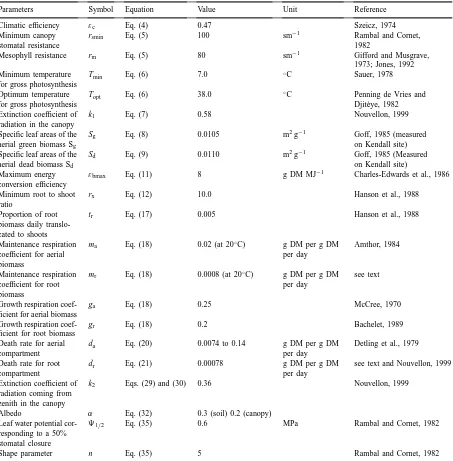
ing the monsoon precipitation of 1990 and 1991, it can be noted that the 1990 precipitation pattern was more favourable to plant growth due to both its higher amount and its distribution pattern. For year 1992, it should be noted that rainfall during the spring was higher than normal. The VPD was less during the 1990
monsoon season than during the two other monsoon seasons.
Fig. 1. Measured daily rainfall and vapour pressure deficit.
year 1991 and 1992, that is 47% of the total incident radiation.
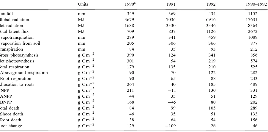
Simulated daily transpiration, soil evaporation and evapotranspiration are shown in Fig. 2. Daily ET was highly variable due to the variation of potential evap-otranspiration (PET (Lhomme, 1997)) and soil wa-ter availability. Due to the low plant fractional cover, transpiration was generally less than soil evaporation. From June 28 1990 through the end of 1992, accumu-lated transpiration, evaporation and actual evapotran-spiration were 212, 877 and 1089, respectively. Thus, the model predicted that evaporation represented 80% of the ET, while transpiration represents only 20% of total ET. Deep drainage below 0.60 m was predicted to be only 5% of total precipitation.
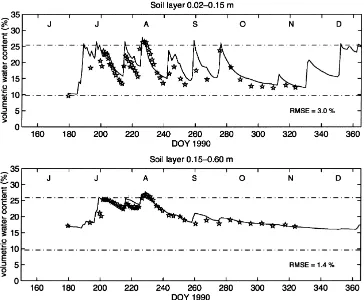
Simulated soil water content in layers 2–15 and 15–60 cm are shown in Fig. 3 for year 1990. Compari-son with measurements showed that soil water content was well simulated and soil water regime generally
followed the patterns described by Herbel and Gibbens (1987).
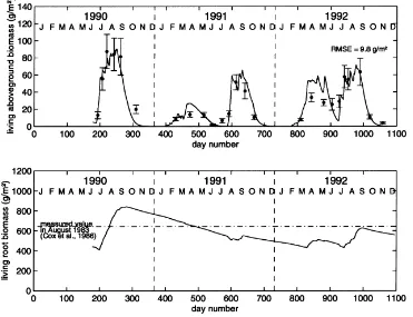
Simulated living aboveground biomass and living root biomass are shown in Fig. 4. Results show that living aboveground biomass simulations closely fol-lowed measurements with an overestimation during spring, 1992. This could have been caused by the in-ability of the model to account for small changes in the floristic composition of the vegetation canopy and particularly the presence of C3and C4annual grasses
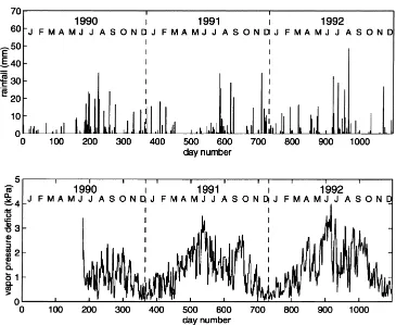
Table 2
Terms of the water, energy and carbon budgets for three consecutive years (g C m−2 are obtained from g DM m−2 by dividing by 2.5, considering biomass is mainly composed of (CH2O)n)
Units 1990a 1991 1992 1990–1992
Rainfall mm 349 369 434 1152
Global radiation MJ 3679 7036 6916 17631
Net radiation MJ 1688 3330 3346 8364
Total latent flux MJ 709 837 1126 2672
Evapotranspiration mm 289 341 459 1089
Evaporation from soil mm 205 306 366 877
Transpiration mm 84 35 93 212
Gross photosynthesis g C m−2 390 124 341 856
Net photosynthesis g C m−2 301 54 219 574
Total respiration g C m−2 179 135 210 525
Aboveground respiration g C m−2 90 70 122 282
Root respiration g C m−2 90 65 88 243
Allocation to roots g C m−2 264 40 185 489
TNPP g C m−2 211 −11 130 331
ANPP g C m−2 44 35 51 129
BNPP g C m−2 168 −45 80 202
Total death g C m−2 84 99 105 289
Shoot death g C m−2 46 35 51 133
Root death g C m−2 38 64 54 156
Root change g C m−2 129
−109 26 46
aFrom June 28.
season. For each year, peak biomass was obtained in mid-September (90 g DM m−2in 1990; 65 g DM m−2
in 1991; and 72 g DM m−2 in 1992). The highest
yield, obtained in summer 1990, was produced by a favourable pattern of rainfall.
Root biomass decreases between growing seasons due to respiration and senescence. This decrease is accelerated during the start of vegetation growth in Spring and Summer due to translocation of carbohy-drates from roots to young shoots. After shoot devel-opment, when the amount of photoassimilated carbon allocated from the shoots to roots exceed root res-piration and senescence, root biomass increases, and reaches its maximum value at the end of the growing season (end of September/beginning of October). Root biomass increase was very high during the monsoon season of 1990, but moderate in 1992 and negligible in 1991.
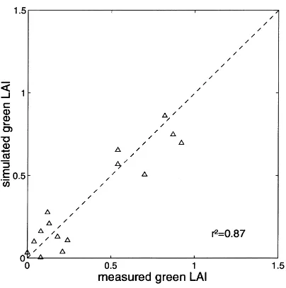
Maximum LAI for monsoon seasons 1990–1992 were 0.94, 0.68 and 0.74, respectively. Regression analysis showed that simulated and measured green LAI compared well with a coefficient of determina-tion of 0.87 (Fig. 5).
Results for the carbon budget are shown in Table 2. Gross and net photosynthesis were highly variable
from 1 year to the next. In 1990, gross photosynthe-sis was 3.1 times that of year 1991. The variability of simulated Aboveground Net Primary Productivity (ANPP) was much less than that of simulated gross and net photosynthesis, explained by the fact that the years with higher amounts of gross photosynthesis were also those with higher allocation of carbon to the roots. Simulated Belowground Net Primary Pro-ductivity (BNPP) for year 1991 was negative because simulated carbon allocation to the roots was lower than that consumed in respiration or translocated to the shoots. Root respiration is the sum of growth res-piration and maintenance resres-piration and thus depends on the amount of carbon allocated to the roots and the root biomass. For years 1990 and 1992, higher alloca-tion to the roots led to a higher root growth respiraalloca-tion and total root respiration.
4. Discussion
Fig. 2. Simulated daily (a) total evaporation, (b) evaporation from soil, and (c) transpiration.
evaporation processes used on average 32% of the net radiation. The amount of transpiration was found to be low when compared to evaporation. On an annual basis, modelled transpiration represented only 20% of actual evapotranspiration because of the low fractional cover of green vegetation even during the growing sea-son. Furthermore, this region is often characterised by small inefficient rain events that wet only the surface soil layer.
Mean annual ANPP and TNPP (Aboveground and Total Net Primary Productivity) were 107 and 276 g DM m−2, respectively. Thus, the ratio of ANPP/TNPP was 0.39. For semi-arid grasslands, values for this ra-tio range between 0.25 and 0.6 (Sims and Singh, 1978; Milchunas and Lauenroth, 1992). Over the 3 years, 57% of gross photosynthesis and 85% of net photo-synthesis were allocated to roots. This is consistent with the simulation results of Detling et al. (1979) who found that 65% of Pgand 80% of Pnwere
allo-cated to belowground structures. Sixty-one percent of
Pg was lost in total respiration, a value close to that
found by Detling et al. (1979). Root respiration repre-sented 46% of total respiration, an intermediate value between the lowest 21% found by Bachelet (1989) and the highest 71% by Detling et al. (1979). The amount lost by aboveground respiration was 33% of Pg.
Fig. 3. Volumetric soil water content of layers 0.02–0.15 and 0.15–0.60 m. Solid lines refer to simulations and stars refer to measurements. Broken lines show field capacity and air dryness.
proportion of assimilate allocation to the roots, and the carbon losses due to respiration. This efficiency was 0.29 g DM (MJ IPAR)−1 (equivalent to 0.12 g C (MJ IPAR)−1). This value was in the lower range of those found by Paruelo et al. (1997), in 19 sites of the central grassland region of the United States. The conversion efficiencies found by Paruelo et al. (1997) varied between 0.1 g C (MJ IPAR)−1 for the least productive sites to 0.20 g C (MJ IPAR)−1for the most productive sites.
Water Use Efficiency (WUE) is an interesting in-dicator of the efficiency with which scarce water resources are used by plants in arid or semiarid en-vironments. WUE was defined here as the ratio of ANPP or TNPP to the total water evapotranspired or transpired during a given period of time. Most of the WUE values given in the literature for natural ecosys-tems were calculated as the ratio of ANPP/AET, due
to the difficulty of estimating BNPP and transpiration. Values obtained for shortgrass prairies of the United States usually range between 0.2 and 0.7 g DM kg−1 evapotranspirated H2O (e.g. Webb et al., 1978;
Fig. 4. Time course of simulated (a) living aboveground biomass and (b) living root biomass compared to measurements.
which in turn increased the transpiration/AET ratio and consequently the WUE. This result was consistent with those found by Liang et al. (1989) and is called the inverse texture effect. Sala et al. (1988) found that when precipitation was less than 370 mm per year in North American semi-arid grasslands, sandy soils with low field capacity and low water-holding capac-ity were more productive than loamy soils with high water-holding capacity, while the opposite pattern occurred when precipitation was more than 370 mm.
When WUE is defined as the ratio of TNPP/AET (WUE–TNPP), an annual value of 0.76 was obtained while a value of 1.05 was found when only the growing season was considered. The values obtained by Sims and Singh (1978) over the growing season on a desert grassland range between 0.87 and 2.07.
Transpiration Use Efficiency (TUE) can be de-fined as the ratio of net production/transpiration. We obtained TUE–ANPP of about 1.52 g DM kg−1 tran-spired H2O and TUE–TNPP of about 3.93 on an
annual basis, or 4.37 for the growing season. The
TUE–ANPP obtained was higher than that reported by Aguiar et al. (1996) (1.07 g DM kg−1 transpired H2O), but similar to those of Downes (1969) who
found 1.49 for grasses. The TUE–TNPP values ob-tained were higher than those found by Dwyer and De Garmo (1970) (2.29 g DM kg−1H2O for B. eriopoda
Torr. and Hilaria mutica (Bckl.) Benth.), but lower than those found by Wright and Dobrenz (1973) for different lines of Eragrostis lehmanniana Nees (be-tween 5.62 and 7.41 g DM kg−1 H
2O depending on
the line).
5. Conclusions and further developments
Fig. 5. Comparison of simulated and measured green LAI (1990–1991).
consecutive years with contrasting rainfall patterns and biomass productions were used to validate the model. It was shown that the model was capable of adequately reproducing the time course of biomass, LAI, and soil water content for the three consecutive growing seasons without interruption. Furthermore, other state variables or terms of the water and carbon budgets (e.g. transpiration) which could not be directly compared to field measurements, have been compared with re-sults of previous works carried out on similar ecosys-tems. This indicated an overall consistency between results of the model simulations and results of other studies.
Estimates of biomass production and evapotran-spiration fluxes at a regional scale are important information for rangeland management. However, the application of simulation models for that purpose could be undermined by spatially unknown parame-ters such as rooting depth, or initial conditions such as root biomass, and climatic data such as rainfall, to which model simulations can be moderately to highly sensitive. At that scale, the spatial and tem-poral information provided by satellite sensors could prove valuable, and an assessment of the possibility of combining remote sensing data and model simu-lations is being carried out (Nouvellon et al., 1998, 1999).
Acknowledgements
The authors wish to thank USDA-ARS for provid-ing the data set. This research activity has been carried out in the framework of SALSA-Experiment (NASA grant W-18, 997), Monsoon’90 (IDP-88-086), VEG-ETATION (58-5344-6-F806 95/CNES/0403), and Landsat7 (NASA-S-1396-F) projects. Thanks also to Philip Heilman and Scott Miller of USDA, and to two anonymous reviewers, for their comments which helped us to improve an earlier version of the paper.
References
Aguiar, M.R., Paruelo, J.M., Sala, O.E., Lauenroth, W.K., 1996. Ecosystem responses to changes in plant functional type composition: an example from the Patagonian steppe. J. Veg. Sci. 7, 381–390.
Ahuja, L.R., Naney, J.W., Williams, R.D., 1985. Estimating soil water characteristics from simpler properties or limited data. Soil Sci. Soc. Am. J. 49, 1100–1105.
Amer, S.A., Keefer, T.O., Weltz, M.A., Goodrich, D.C., Bach, L.B., 1994. Soil moisture sensors for continuous monitoring. Water Resour. Bull. 30 (1), 69–83.
Anway, J.C., Brittain, E.G., Hunt H.W., Innis, G.S., Parton, W.J., Rodell, C.F., Sauer, R.H., 1972. ELM: Version 1.0. Grassland Biome-US. International Biological Program Tech. Rep. No. 156. Colorado State University, Fort Collins.
Amthor, J.S., 1984. The role of maintenance respiration in plant growth. Plant Cell Environ. 7, 561–569.
Arya, L.M., Paris, J.F., 1981. A physicoempirical model to predict the soil moisture characteristics from particle-size distribution and bulk density data. Soil Sci. Soc. Am. J. 45, 1023–1030. Bachelet, D., 1989. A simulation model of intraseasonal carbon
and nitrogen dynamics of blue grama swards as influenced by above-and belowground grazing. Ecol. Modell. 44, 231–252. Branson, F.A., Gifford, G.F., Owen, R.J., 1972. Rangeland
hydrology. Range Sci. Ser., Soc. for Range Manage., Denver, Colorado, p. 84.
Brooks, R.H., Corey, A.T., 1964. Hydraulic properties of porous media. Hydrology paper 3, Colorado State University, Fort Collins.
Camillo, P.J., Gurney, R.J., 1986. A resistance parameter for bare soil evaporation models. Soil Sci. 141, 95–105.
Campbell, G.S., 1974. A simple method for determining unsaturated conductivity from moisture retention data. Soil Sci. 117, 311–314.
Charles-Edwards, D.A., Doley, D., Rimmington, G.M., 1986. Modelling Plant Growth and Development. Academic Press, Orlando, FL.
Clapp, R.B., Hornberger, G.M., 1978. Empirical equations for some hydraulic properties. Water Resour. Res. 14, 601–604. Clark, F.E., Paul, E.A., 1970. The microflora of grassland. Adv.
Agron. 22, 375–435.
Coughenour, M.B., McNaughton, S.J., Wallace, L.L., 1984. Modelling primary production of perennial graminoids — uniting physiological processes and morphometric traits. Ecol. Modell. 23, 101–134.
Cox, J.R., Frasier, G.W., Renard, K.G., 1986. Biomass distribution at Grassland and Shrubland sites. Rangelands 8 (2), 67–68. De Jong, R., 1983. Soil water description curves estimated from
limited data. Can. J. Soil Sci. 63, 697–703.
Detling, J.K., Parton, W.J., Hunt, H.W., 1979. A simulation model of Bouteloua gracilis biomass dynamics on the North American shortgrass prairie. Oecologia 38, 167–191.
Downes, R.W., 1969. Differences in transpiration rates between tropical and temperate grasses under controlled conditions. Planta 88, 261–273.
Dunkerley, D.L., Booth, T.L., 1999. Plant canopy interception of rainfall and its significance in a banded landscape, arid western New South Wales, Australia. Water Resour. Res. 35 (5), 1581– 1586.
Dwyer, D.D., De Garmo, H.C., 1970. Greenhouse productivity and water use efficiency of selected desert shrubs and grasses under four soil-moisture levels New Mexico State University, Agric. Exp. Stat. Bull. 570, Las Cruces, New Mexico. Feddes, R.A., Kowalik, P.J., Zaradny H., 1978. Simulation of field
water use and cropyield. Simulation Monograph. Pudoc-DLO, Wageningen, The Netherlands, p. 189.
Gifford, R.M., Musgrave, R.B., 1973. Stomatal role in the variability of net CO2 exchange rate by two maize inbreds. Aust. J. Biol. Sci. 26, 35–44.
Goff, B.F., 1985. Dynamics of canopy structure and soil surface cover in a semi-arid grassland. Master’s thesis, University of Arizona, Tucson.
Goodrich, D.C., 1994. SALSA-MEX: A large scale Semi-Arid Land-Surface-Atmospheric Mountain Experiment. In: Proc. Int. Geoscience and Remote Sensing Symp. (IGARSS’94), Pasadena, CA, vol. 1, August 8–12, 1994, pp. 190–193. Goodrich, D.C., Chehbouni, A.G., Goff, B. et al., 1998.
An overview of the 1997 activities of the Semi-Arid Land-Surface-Atmosphere (SALSA program). Proc. 78th American Meteorological Society Annual Meeting, Phoenix, Arizona, 11–16 January.
Hanson, J.D., Parton, W.J., Innis, G.S., 1985. Plant growth and production of grassland ecosystems: a comparison of modelling approaches. Ecol. Modell. 29, 131–144.
Hanson, J.D., Skiles, J.W., Parton, W.J., 1988. A multi-species model for rangeland plant communities. Ecol. Modell. 44, 89– 123.
Herbel, C.H., Gibbens, R.P., 1987. Soil water regimes of loamy sands and sandy loams on arid rangelands in southern New Mexico. J. Soil Water Conserv. 42, 442–447.
Jones, H.G., 1992. Plants and Microclimate. A Quantitative Approach to Environmental Plant Physiology, 2nd ed. Cambridge University Press, Cambridge, p. 429.
Kowalik, P.J., Turner, N.C., 1983. Diurnal changes in the water relations and transpiration of a soybean crop simulated during the development of water deficits. Irrig. Sci. 4, 225–238. Kustas, W.P., Goodrich, D.C., 1994. Preface to the special issue
on Monsoon 90. Water Resour. Res. 30 (5), 1211–1225. Kustas, W.P., Blanford, J.A., Stannard, D.I., Daughtry, C.S.T.,
Nichols, W.D., Weltz, M.A., 1994. Water Resour. Res. 30 (5), 1351–1361.
Lapitan, R.L., Parton, W.J., 1996. Seasonal variabilities in the distribution of the microclimatic factors and evapotranspiration in a shortgrass steppe. Agric. For. Meteorol. 79, 113–130. Lauenroth, W.K., 1979. Grassland primary production:
North American grasslands in perspective. In: French, N.L. (Ed.), Perspectives in Grassland Ecology. Springer, Berlin/Heidelberg/New York, pp. 2–24.
Leenhardt, D., Voltz, M., Rambal, S., 1995. A survey of several agroclimatic soil water balance models with reference to their spatial application. Eur. J. Agron. 4, 1–14.
Le Houérou, H.N., 1984. Rain use efficiency: a unifying concept in arid-land ecology. J. Arid Environ. 7, 213–247.
Liang, Y.M., Hazlett, D.L., Lauenroth, W.K., 1989. Biomass dynamics and water use efficiencies of five plant communities in the shortgrass steppe. Oecologia 80, 148–153.
Lhomme, J.P., 1997. Towards a rational definition of potential evaporation. Hydrol. Earth System Sci. 1 (2), 257–264. Lo Seen, D., Mougin, E., Rambal, S., Gaston, A., Hiernaux,
P., 1995. A regional Sahelian grassland model to be coupled with multispectral satellite data. II. Toward the control of its simulations by remotely sensed indices. Remote Sens. Environ. 52, 194–206.
Lo Seen, D., Chehbouni, A., Njoku, E., Saatchi, S., Mougin, E., Monteny, B., 1997. An approach to couple vegetation functioning and soil-vegetation-atmosphere-transfer models for semiarid grasslands during the HAPEX-Sahel experiment. Agric. For. Meteorol. 83, 49–74.
McCree, K.J., 1970. An equation for the rate of respiration of white clover plants grown under controlled conditions. In: Setlik, I. (Ed.), Prediction and Measurement of Photosynthetic Productivity. Proc. IBP/PP Tech. Meet., Trebon. PUDOC, Wageningen, The Netherlands, pp. 221–229.
Mc Mahon, J.A., Wagner, F.H., 1985. The Mojave, Sonoran and Chihuahuan deserts of North America. In: Evenari, M., Noy-Meir, I., Goodall, D.W. (Eds.), Hot Deserts and Arid Shrublands. Ecosystems of the world 12A, pp. 105–202. Milchunas, D.G., Lauenroth, W.K., 1992. Carbon dynamics and
estimates of primary production by harvest,14C dilution, and 14C turnover. Ecology 73 (2), 593–607.
Monteith, J.L., 1965. Evaporation and the environment. Symp. Soc. Exp. Biol. 19, 205–234.
Mougin, E., Lo Seen, D., Rambal, S., Gaston, A., Hiernaux, P., 1995. A regional Sahelian grassland model to be coupled with multispectral satellite data. I. Model description and validation. Remote Sens. Environ. 52, 181–193.
Nouvellon, Y., Lo Seen, D., Bégué, A., Rambal, S., Moran, M.S., Qi, J., Chehbouni, A., Kerr, Y., 1998. Combining remote sensing and vegetation growth modeling to describe the carbon and water budget of semi-arid grasslands. IGARSS’98, 6–10 July, Seattle, Washington.
Nouvellon, Y., Lo Seen, D., Rambal, S., Bégué, A., Moran, M.S., Kerr, Y., Qi, J., 1999. Time course of radiation use efficiency in a shortgrass ecosystem: consequences for remotely-sensed estimation of primary production. Remote Sens. Environ., in press.
Osborn, H.B., Lane, L.J., Hundley, J.F., 1972. Optimum gaging of thunderstorm rainfall in Southeastern Arizona. Water Resour. Res. 8 (1), 259–265.
Paruelo, J.M., Epstein, H.E., Lauenroth, W.K., Burke, I.C., 1997. ANPP estimates from NDVI for the central grassland region of the United States. Ecology 78 (3), 953–958.
Penning de Vries, F.W.T., Djitèye, M.A., 1982. La productivité des pâturages Sahéliens. Une étude des sols, des végétations et de l’exploitation de cette ressource naturelle. Agric. Res. Rep. 918, Pudoc, Wageningen, p. 525.
Perrin de Brichambaut, C., Vauge, C., 1982. Le gisement solaire. Evaluation de la ressource énergétique. Lavoisier Ed., Paris. Rambal, S., Cornet, A., 1982. Simulation de l’utilisation de l’eau
et de la production végétale d’une phytocénose Sahélienne du Sénégal. Acta Oecologica Oecol. Plant 3 (17), 381–397. Rawls, W.J., Brakensiek, D.L., Saxton, K.E., 1982. Estimation of
soil water properties. Transac. Am. Soc. Agric. Eng. 25, 1316– 1320.
Renard, K.G., Lane, L.J., Simanton, J.R., Emmerich, W.E., Stone, J.J., Weltz, M.A., Goodrich, D.C., Yakowitz, D.S., 1993. Agricultural impacts in an arid environment: Walnut Gulch studies. Hydrol. Sci. Technol. 9 (1–4), 145–190.
Ruimy, A., Dedieu, G., Saugier, B., 1996. TURC: a diagnostic model of continental gross primary productivity and net primary productivity. Glob. Biogeochem. Cycles 10, 269–286. Sala, O.E., Parton, W.J., Joyce, L.A., Lauenroth, W.K., 1988.
Primary production of the central grassland region of the United States. Ecology 69 (1), 40–45.
Sauer, R.H., 1978. A simulation model for grassland primary producer phenology and biomass dynamics. In: Innis, G.S. (Ed.), Grassland Simulation Model. Ecological Studies, 26. Springer, Berlin/Heidelberg/New York, pp. 55–87.
Saxton, K.E., Rawls, W.J., Romberger, J.S., Papendick, R.I., 1986. Estimating generalized soil-water characteristics from texture. Soil Sci. Soc. Am. J. 50, 1031–1036.
Sellers, W.D., Hill, R.H., 1974. Arizona climate 1931–1972. The University of Arizona Press, Tucson.
Sims, P.L., Singh, J.S., 1978. The structure and the function of ten western north american grasslands. III. Net primary production. Turnover and efficiencies of energy capture and water use. J. Ecol. 66, 573–597.
Singh, J.S., Coleman, D.C., 1975. Evaluation of functional root biomass and translocation of photoassimilated carbon-14 in a shortgrass prairie ecosystem. In: Marshall, J.K. (Ed.), The Belowground Ecosystem: A Synthesis of Plant Associated Processes. Dowden, Hutchison and Ross, Stroudsburg, Pennsylvania.
Shuttleworth, W.J., 1993. Evaporation. In: Maidment, D.R. (Ed.), Handbook of Hydrology. McGraw-Hill, New York.
Stannard, D.I., Blanford, J.H., Kustas, W.P., Nichols, W.D., Amer, S.A., Schmugge, T.J., Weltz, M.A., 1994. Interpretation of surface flux measurements in heterogeneous terrain during the Monsoon ’90 experiment. Water Resour. Res. 30 (5), 1227– 1239.
Szeicz, G., 1974. Solar radiation for plant growth. J. Appl. Ecol. 11, 617–636.
Tiscareno-Lopez, M., 1994. A bayesian-monte carlo approach to access uncertainties in process-based, continuous simulation models. Ph.D. thesis, University of Arizona, Tucson. Thurow, T.L., Blackburn, W.H., Warren, S.D., Taylor, C.A., 1987.
Rainfall interception by midgrass, shortgrass, and live oak mottes. J. Range Manage. 40, 455–460.
Van Keulen, H., 1975. Simulation of water use and herbage growth in arid regions. Simulation Monographs. Pudoc, Wageningen, p. 176.
Webb, W., Szarek, S., Lauenroth, W., Kinerson, R., Smith, M., 1978. Primary productivity and water use in native forest, grassland, and desert ecosystems. Ecology 59 (6) 1239–1247.
Weltz, M.A., Ritchie, J.C., Fox, H.D., 1994. Comparison of laser and field measurements of vegetation height and canopy cover. Water Resour. Res. 30 (5), 1311–1319.
White, E.G., 1984. A multispecies simulation model of grassland producers and consumers II. Producers. Ecol. Modell. 24, 241– 262.