MULTISPECTRAL AIRBORNE LASER SCANNING
FOR AUTOMATED MAP UPDATING
Leena Matikainen*, Juha Hyyppä, Paula Litkey
Finnish Geospatial Research Institute FGI, Centre of Excellence in Laser Scanning Research, at the National Land Survey of Finland, Geodeetinrinne 2, FI-02430 Masala, Finland – (leena.matikainen, juha.hyyppa, paula.litkey)@nls.fi
KEY WORDS: Laser scanning, Lidar, Multispectral, Point cloud, Mapping, Automation, Updating, Change detection
ABSTRACT:
During the last 20 years, airborne laser scanning (ALS), often combined with multispectral information from aerial images, has shown its high feasibility for automated mapping processes. Recently, the first multispectral airborne laser scanners have been launched, and multispectral information is for the first time directly available for 3D ALS point clouds. This article discusses the potential of this new single-sensor technology in map updating, especially in automated object detection and change detection. For our study, Optech Titan multispectral ALS data over a suburban area in Finland were acquired. Results from a random forests analysis suggest that the multispectral intensity information is useful for land cover classification, also when considering ground surface objects and classes, such as roads. An out-of-bag estimate for classification error was about 3% for separating classes asphalt, gravel, rocky areas and low vegetation from each other. For buildings and trees, it was under 1%. According to feature importance analyses, multispectral features based on several channels were more useful that those based on one channel. Automatic change detection utilizing the new multispectral ALS data, an old digital surface model (DSM) and old building vectors was also demonstrated. Overall, our first analyses suggest that the new data are very promising for further increasing the automation level in mapping. The multispectral ALS technology is independent of external illumination conditions, and intensity images produced from the data do not include shadows. These are significant advantages when the development of automated classification and change detection procedures is considered.
* Corresponding author
1. INTRODUCTION
During the last 20 years, airborne laser scanning (ALS) has shown its high feasibility for automated mapping processes. The accurate 3D data, often combined with spectral information from digital aerial images, have allowed the development of methods for automated object extraction and change detection. In particular, important advancements have been achieved in the mapping of elevated objects such as buildings and trees (e.g., Hug, 1997; Rottensteiner et al., 2007; Guo et al., 2011).
In addition to 3D modelling of objects, an important application area of ALS data has been automated change detection. Methods developed for change detection of buildings can be roughly divided into two groups based on the input data available. The first group uses new ALS data, possibly combined with new image data, and aims to detect changes compared to an existing building map (e.g., Matikainen et al., 2003, 2010; Vosselman et al., 2005; Malpica et al., 2013). The second approach assumes that both old and new ALS datasets are available and the change detection method can rely on the comparison of these (e.g., Murakami et al., 1999; Richter et al., 2013; Teo and Shih, 2013). In the first group of methods, the methods are directly linked to the existing building objects on a map, and change information is normally obtained for these objects. In the second group, the link between the change detection method and existing building maps or models is often weaker.
The role of laser intensity has been relatively small in the development of object detection and change detection methods. Intensity information, increasingly also from full-waveform
data, has been used in many classification studies (e.g., Hug, 1997; Guo et al., 2011), but generally the geometric information of the laser scanner data has been more important. In 2008, EuroSDR (European Spatial Data Research) initiated a project ‘Radiometric Calibration of ALS Intensity’ lead by the Finnish Geospatial Research Institute FGI and TU Wien in order to increase the awareness of intensity calibration. It was expected that someday multispectral ALS is available and then intensity of ALS will be of high value. Thus, earlier intensity studies (e.g., Ahokas et al., 2006; Höfle and Pfeifer, 2007) showing the concepts for radiometric calibration of ALS intensity, have been preparations for multispectral ALS.
Laser scanning systems providing geometric and multispectral information simultaneously provide interesting possibilities for further development of automated object detection and change detection. Experiences on this field have been obtained, for example, from studies with a hyperspectral laser scanner developed at the FGI (Chen et al., 2010; Hakala et al., 2012). The system is a terrestrial one and has been successfully applied for vegetation analyses and separation of man-made targets from natural ones (e.g., Puttonen et al., 2015). Phennigbauer and Ullrich (2011) discussed the development and potential of multi-wavelength ALS systems. Briese et al. (2013) realized such an approach by using three separate ALS systems. The study concentrated on radiometric calibration of intensity data from an archaeological study area. Wang et al. (2014) used two separate ALS systems to acquire dual-wavelength data for classifying land cover. They found that the use of dual-wavelength data can substantially improve classification accuracy compared to one-wavelength data. More extensive discussions and reference lists on these earlier developments of The International Archives of the Photogrammetry, Remote Sensing and Spatial Information Sciences, Volume XLI-B3, 2016
multispectral laser scanning can be found, for example, in Puttonen et al. (2015) and Wichmann et al. (2015).
The first operational multispectral ALS system was launched by Teledyne Optech (Ontario, Canada) in January 2015 with the product name Titan. With this scanner, multispectral information is for the first time directly available for 3D ALS point clouds. The first studies based on Optech Titan data have been published. Wichmann et al. (2015) used data from Ontario, Canada, obtained with a prototype of the system, and evaluated the potential of the data for topographic mapping and land cover classification. They analysed spectral patterns of land cover classes and carried out a classification test. The analysis was point-based and used a single point cloud that was obtained by merging three separate point clouds from the three channels by a nearest neighbour approach. The intensity information was not calibrated. Wichmann et al. (2015) concluded that the data are suitable for conventional geometrical classification and that additional classes such as sealed and unsealed ground can be separated with high classification accuracies using the intensity information. They also discussed multi-return and drop-out effects (drop-outs referred to cases where returns are not obtained in all channels). For example, the spectral signature of objects such as trees becomes biased due to multi-return effects. Bakula (2015) also used Optech Titan testing data from Ontario. Digital surface models (DSMs) and digital terrain model (DTMs) created separately from the different channels were analysed. Differences occurred in vegetated areas and building edges due to various distributions of points. For DTMs, the differences were small. Bakula (2015) also showed intensity images created in raster format, a classification result produced in Terrasolid software, and scatter plots illustrating the intensity values in a few classes.
Our article discusses the potential of this new single-sensor technology in map updating, especially in automated object detection and change detection. For our study, Optech Titan multispectral ALS data over a large suburban area in Finland were acquired. The data were acquired with an operational system, i.e., we did not use testing data. In this article, we will present the first results of automated object detection by applying the data. In particular, our objective was to study how the novel multispectral information can benefit land cover mapping. An object-based approach using rasterized data was used. Averaging of intensity data diminishes possible problems related to individual intensity values and helps to give an overall understanding of the capabilities of the new data. In addition, change detection of buildings will be demonstrated. In this case, we consider a “second-generation” ALS-based map updating approach where two ALS datasets are available: an old one based on conventional one-channel ALS and a new one from multispectral ALS. This is likely to become a realistic situation in many mapping organizations during the following years. The change detection approach exploits the possibility to compare the old and new datasets, but it also uses the multispectral data and it is directly linked to the existing building vectors.
2. DATA
2.1 Multispectral ALS data
Multispectral Optech Titan data were acquired on 21 August 2015 in cooperation with TerraTec Oy (Helsinki, Finland). The flying altitude was about 650 m above sea level. The scanned
area included southern parts of the city of Espoo, next to Helsinki, and it covers about 50 km2 in total. In this article, we concentrate on analysing a suburban area of 4 km2 in Espoonlahti. The dataset includes three channels available as separate point clouds (Ch1: infrared, 1550 nm; Ch2: near-infrared, 1064 nm; Ch3: green, 532 nm). The point density in one channel is about 6 points/m2, resulting in a total density of about 18 points/m2.
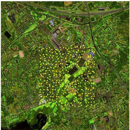
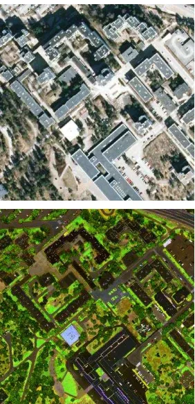
The first part of preprocessing was carried out by TerraTec Oy and included some basic processing steps such as geoid correction and strip matching. Further processing was carried out at the FGI. A range correction was applied to the intensity information to make relative radiometric calibration (Ahokas et al., 2006; Kaasalainen et al., 2011). As expected, our preliminary analyses with uncorrected data showed that intensity values were highest in the middle of a flight line and decreased as the distance from the scanner increased. After the radiometric correction, functions of TerraScan software (Terrasolid Ltd., Helsinki, Finland) were used to cut overlap points and remove erroneously high or low points. Finally, three-channel intensity images and DSMs in raster format were created. In the intensity images, pixel values in each channel represent the average intensity value of first pulse and only pulse laser points in the corresponding channel. For creating the DSMs, a combined point cloud from all channels was used. Maximum and minimum DSMs, presenting the highest or lowest height within the pixel, respectively, were created. The pixel size of the intensity images used in the present study was 20 cm. The pixel size of the DSMs was 1 m. For the intensity images, the small pixel size was preferred to better represent small details such as narrow roads. For the DSMs, the larger pixel size appeared advantageous to avoid some noise in building edges and to remove most of the vegetation from the minimum DSMs. Figure 1 shows a three-channel intensity image covering the study area discussed in this article. In Figure 2, the intensity image can be compared with a conventional aerial ortho image. It should be noted, however, that the acquisition time of the images was different. In the Titan data, deciduous trees are in full leaf, while the aerial ortho image is from leaf-off conditions in early spring.
Figure 1. Three-channel intensity image of the 2 km × 2 km study area (Channels 1–3 in red, green and blue, respectively). Reference points used in the analysis are shown on the image. The International Archives of the Photogrammetry, Remote Sensing and Spatial Information Sciences, Volume XLI-B3, 2016
Figure 2. Comparison of an aerial ortho image and Titan intensity image in a 300 m × 300 m subarea. Ortho image © National Land Survey of Finland, 2013.
2.2 Reference points
A land cover classification test field established previously was used as reference data (see Matikainen and Karila, 2011). A set of 332 reference points was used in the present study. The location and land cover of these points was checked and updated to correspond to the current situation. The updating was based on visual interpretation of the Titan data and open datasets available from the National Land Survey of Finland (NLS), the City of Espoo, Google Maps (https://maps.google.com) and Google Street View. Field checks were used to support the analysis and to check uncertain cases. The reference points basically have information on object types and surface types. For the present study, the information was generalized to the following classes:
Building (88 points): Different types of buildings (e.g., high-rise residential, low-rise residential, public) with different roof materials and colours are included.
Tree (81 points): Includes coniferous and deciduous trees in forest, in gardens and along roads.
Asphalt (62 points): In addition to 58 asphalt points, 4 road or parking place points with tile surface were included. Gravel (15 points): Includes soft, non-vegetated surfaces
with different grain sizes.
Rocky area (16 points): Includes rocky areas with bare or slightly vegetated surface (typically some moss).
Low vegetation (70 points): This class includes grass (19 points), meadow (31), forest floor (4), vegetable gardens (9), and low bushes (7). The sub-classes were combined due to the small number of points in a class or uncertainty in separating the classes even in field checks (grass and meadow).
Water areas were excluded from the analysis by using a water mask derived from topographic map data.
2.3 Old building map and old DSM
A building map representing the situation in 2005 was used as an old map in change detection. The data were originally obtained from the City of Espoo and edited at the FGI to correspond to the situation in 2005. An old DSM based on Optech ALTM 3100 ALS data acquired in 2005 was also used as input data in the change detection. The DSM represented the minimum height values for 0.3 m × 0.3 m pixels. More detailed descriptions of these old datasets can be found in Matikainen et al. (2010).
2.4 DTM
As DTM, we used a national DTM produced by the NLS. A similar DTM could have been derived from the Titan data, but since in complex suburban areas, there are some areas needing manual editing, an existing DTM was applied. The NLS DTM is available in raster format, and it has a pixel size of 2 m × 2 m. The DTM is based on national laser scanner data with a minimum point density of 0.5 points/m2. The production process includes automatic classification and manual corrections also using aerial images (NLS, 2016).
3. METHODS
3.1 Land cover classification
Our main interest in this study was to investigate the usefulness of multispectral ALS features in land cover classification. The DSM and intensity image data were first segmented into homogeneous regions, and various attributes (features) were calculated for the segments. These steps were carried out by using the eCognition software (Trimble Germany GmbH, Munich) and its multiresolution segmentation algorithm (Baatz and Schäpe, 2000). The reference points were used to determine training segments for different land cover classes. The potential of the features for separating the classes were then investigated by using histograms and machine learning analyses with the random forests method. Functions of the Matlab software (The Mathworks, Inc., Natick, MA, USA) and its Statistics and Machine Learning Toolbox were used for this purpose.
The random forests method (Breiman, 2001; Breiman and Cutler, 2004) is a further development of classification trees (Breiman et al., 1984), and it belongs to ensemble classification methods. The basic classification tree algorithm creates one classification tree automatically based on training data. In the random forests method, a large number of trees is created and the classification result is obtained as a voting result. Each tree is constructed by using part of the training cases (the remaining cases are called out-of-bag data). If a training set has N cases, N cases are selected at random, but with replacement, for creating a tree. At each node of a tree, m variables out of M (the total number of variables) are selected at random and used to find the best split. The trees are not pruned. This approach is known to lead to an accurate classifier, and it also provides the possibility to calculate feature importance and an estimate of the classification error based on the out-of-bag data. The method does not overfit. (Breiman and Cutler, 2004.) Both the classification tree and random forests methods are well suited for classifying data with a large number of features. They do not require separate feature selection or normalization of feature The International Archives of the Photogrammetry, Remote Sensing and Spatial Information Sciences, Volume XLI-B3, 2016
values. Both methods have also been successfully used for classifying ALS data (for application of random forests, see, for example, Guo et al., 2011). In our study, we used the Matlab function ‘fitensemble’ to construct ensembles of classification trees. The functions ‘oobLoss’ and ‘predictorImportance’ were used to calculate the out-of-bag classification error and feature importance, respectively. The classification error was calculated as the fraction of misclassified data. The feature importance analysis is based on changes in the risk due to splits on every predictor (Mathworks, 2015).
Finally, actual land cover classifications for the area under analysis were carried out in eCognition. The Random Trees implementation (OpenCV, 2016) available in the eCognition software was used. High objects (height > 2.5 m) were classified as buildings and trees. Low objects were classified as asphalt, gravel, rocky areas and low vegetation.
3.2 Change detection
A simple change detection procedure using old building vectors, old DSM, new DSM, new intensity image and DTM as input data was developed and implemented in eCognition. The change detection procedure includes the following main steps: Analysis of building segments derived from the old map.
These are classified as OK, demolished or changed by using the DTM and the old and new DSMs. Changed buildings detected at this stage have changes in height.
Detection of new buildings from the new data. This is carried out by segmenting the minimum DSM outside the old buildings and separating buildings from ground and trees by using height and intensity information.
Combination of old and new buildings into a new building level and analysing this level. One building can now contain sub-segments labelled as old and new. This can occur due to real changes such as extension of the building but also because the building in the DSM is typically slightly different from the same building on the map. The final class is determined on the basis of the relative size of the sub-segments. If the final classification is Old building OK, the original shape and size of the building on the map is retained. For new and changed buildings, the shape will be based on the new DSM.
Detailed rules used in our change detection demo will be presented in Section 4.3.
4. RESULTS
4.1 Analysis of class separability and feature importance
Segmentation was first carried out based on the maximum DSM. This DSM shows tree canopies in their full size, and it basically represents the same information as the intensity image that was created from first pulse and only pulse points. Segments were divided into high and low segments based on their mean height (difference between mean values in the maximum DSM and DTM). The threshold value was 2.5 m. Low segments were merged to each other and resegmented based on the three-channel intensity image. Training segments for buildings and trees were then picked from the high segments, and training segments for asphalt, gravel, rocky areas and low vegetation were picked from the low segments. If there was a reference point inside a segment, this segment became a training segment of the corresponding class.
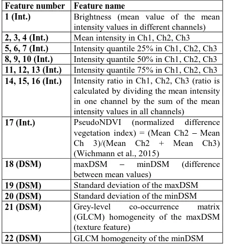
Features selected for the classification analysis and calculated for training segments are shown in Table 1. The importance of the features for separating different classes from each other was tested by analysing different classification cases shown in Table 2. In each case, 1000 classification trees were created, and the out-of-bag classification error and feature importance were calculated. The results are shown in Table 2 and Figure 3. Our main interest was to investigate the intensity features and low level classes that are challenging to distinguish based on one-channel ALS data. In the case of buildings and trees, different feature combinations (intensity or DSM) were tested. In this case, it is well known that DSM data provide useful features, such as the difference between maximum and minimum DSMs and texture features. Here we were interested in studying what is the additional contribution of the multispectral intensity features. Histograms of three most important intensity features are shown for three classification cases in Figure 4.
Feature number Feature name 11, 12, 13 (Int.) Intensity quantile 75% in Ch1, Ch2, Ch3 14, 15, 16 (Int.) Intensity ratio in Ch1, Ch2, Ch3 (ratio is
calculated by dividing the mean intensity in one channel by the sum of the mean intensity values in all channels)
17 (Int.) PseudoNDVI (normalized difference vegetation index) = (Mean Ch2 – Mean Ch 3)/(Mean Ch2 + Mean Ch3) (Wichmann et al., 2015)
18 (DSM) maxDSM – minDSM (difference between mean values)
19 (DSM) Standard deviation of the maxDSM 20 (DSM) Standard deviation of the minDSM 21 (DSM) Grey-level co-occurrence matrix
(GLCM) homogeneity of the maxDSM (texture feature)
22 (DSM) GLCM homogeneity of the minDSM
Table 1. Features used in the classification analysis. “Int.” refers to intensity features and “DSM” refers to DSM features.
Classes to separate Features 1000 classification trees were created based on training data. The International Archives of the Photogrammetry, Remote Sensing and Spatial Information Sciences, Volume XLI-B3, 2016
a) b)
c) d)
Figure 3. Importance of features (see Table 1) in separating different classes from each other. a) Roads etc. (class includes asphalt and gravel), rocky areas, and low vegetation. b) All low classes, i.e., asphalt, gravel, rocky areas, and low vegetation. c) Asphalt and gravel. d) Buildings and trees. Both intensity and DSM features (feature numbers 1–22) were tested case d), while only intensity features (feature numbers 1–17) were tested in the other cases.
Figure 4. Histograms of training segments in different classes. Top: buildings and trees. Middle: roads etc. (class includes asphalt and gravel), rocky areas, and low vegetation. Bottom: asphalt and gravel. For each case, the three most important intensity features according to the feature importance analysis (Table 2, Figure 3) are shown.
4.2 Land cover classification
The actual land cover classification result for the study area is shown in Figure 5. More detailed figures of the results can be found in Ahokas et al. (2016).The segmentation and selection of training segments were carried out as described in Section 4.1. The Random Trees implementation available in eCognition was used to create 1000 trees for classifying high segments into buildings and trees and 1000 trees for classifying low segments into asphalt, gravel, rocky areas and low vegetation. In the classification of high segments, both DSM and intensity features were used. The classification of low segments was based on the intensity features. As a postprocessing step, buildings smaller than 20 m2 were reclassified as tree. Most of such very small buildings are misclassifications.
Figure 5. Result of land cover classification (class High object includes a few very small segments that remained unclassified in further building/tree classification).
4.3 Change detection
The change detection was demonstrated in a smaller area. The results are presented in Figure 6. The rules and threshold values applied in the change detection are listed in the following. DSM_DIF is the absolute value of the difference between the mean heights in the new and old DSMs; h is the height of the segment, i.e., the difference between the mean heights in the new DSM and DTM; Ratio Ch2 is the mean intensity value in Channel 2 divided by the sum of the mean values in all channels. The feature Ratio Ch2 and its threshold value were obtained from the classification tree analysis. Levels refer to segmentation levels. The main steps of the change detection included:
Analysis of building segment level 1 derived from the old map (segments correspond to buildings):
o DSM_DIF ≤ 2.5 m -> Old building OK
o DSM_DIF > 2.5 m and h ≤ 2.5 m -> Old building
demolished
o Otherwise -> Old building changed
Segmentation of the new DSM outside the old buildings and analysis of this DSM segment level (in change detection we used the minimum DSM because it is advantageous in the analysis of buildings).
o h > 2.5 m and Ratio Ch2 < 0.3005144 -> New building Combination of all buildings into building segment level 2
and analysis of this level. Building segments connected to each other were merged to one segment.
o Area < 20 m2 -> unclassified (to remove small
erroneous building segments)
o Relative area of sub-objects Old building demolished ≥ 0.1 -> Old building demolished
o Relative area of sub-objects Old building changed ≥ 0.1 -> Old building changed
o Relative area of sub-objects New building ≥ 0.9 -> New building
o Relative area of sub-objects New building ≥ 0.5 -> Old building changed
o Otherwise -> Old building OK
Finally, the original shape of buildings classified as Old building OK was retained by converting them back to sub-objects and removing building parts classified as New building.
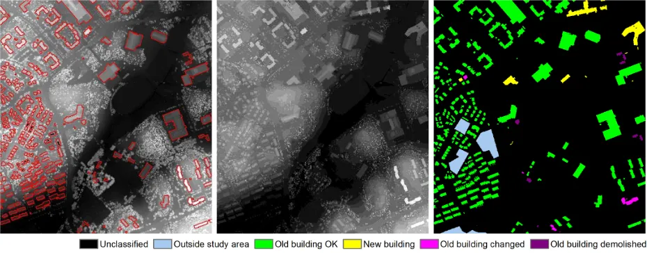
Figure 6. Automated change detection for buildings. The figure shows the old DSM and old building vectors (left), the new DSM (middle), and the change detection result (right). The legend applies to the change detection result. Some areas were excluded from the change detection analysis due to missing data in the old DSM. Original building vectors © the City of Espoo (edited by the FGI).
5. DISCUSSION
Visual analysis of multispectral intensity images produced from the Optech Titan data suggests that the data are very promising for mapping applications, especially considering automated analyses. Unlike conventional passive aerial imaging, the multispectral ALS technology is independent of external illumination conditions, and intensity images produced from the data do not include shadows (see Figure 2). This means a very significant advantage when the development of automated classification and change detection procedures is considered. For example, roads near trees or buildings are better visible on the Titan intensity image than on an aerial ortho image. The direct availability of both geometric and multispectral information from the single sensor also simplifies preprocessing and data analysis workflows.
Results from the random trees analysis clearly support the hypothesis that the multispectral intensity information is useful for land cover classification. Out-of-bag classification errors calculated based on the training data were remarkably small in all tested cases (Table 2). According to the feature importance analysis, features requiring multispectral data, i.e., intensity ratios and PseudoNDVI, were very useful. Some of them always appeared among the most important features.
The results suggest that multispectral ALS data have high potential for separating ground surface classes from each other. Similar results were also reported by Wichmann et al. (2015). In our case, the low classes included asphalt, gravel, rocky areas and low vegetation. These classes cannot be separated on the basis of height data, and results based on one channel intensity data are not likely to be very reliable. For example, as shown in the histograms of Figure 4, asphalt and gravel as one class (roads etc.) were well separated from rocky areas and low vegetation using the feature PseudoNDVI. Rocky areas, on the other hand, were best separated from low vegetation using Ratio Ch2. Useful features for separating asphalt from gravel included Ratio Ch3, Ratio Ch1, and 75% quantile in Ch1. Buildings and trees can be separated from each other by using DSM data. However, also in this case the multispectral feature Ratio Ch2 was clearly the most important feature among the tested ones (Figure 3).
On the basis of visual evaluation, the land cover classification result shown in Figure 5 is relatively good. The most prominent errors are some bridges classified as buildings. This occurred because the DSM and DTM have a clear height difference in these places. The bridges were thus classified as high objects, which were further divided into buildings and trees. Further improvements are needed to avoid such misclassifications. In operational map updating work, use of a road database would be one viable solution. A closer look reveals that smaller errors also occur in the results. Future work should include a detailed analysis of the classification accuracy, preferably in a separate testing area and with a larger number of reference points. The out-of-bag classification error gives an estimate of the classification error, but it should be noted that the number of reference points was relatively small, especially in classes gravel and rocky area. This is likely to have some effect on the results. Our plan is to continue the tests with larger reference datasets. More land cover classes could also be included in the analyses.
Change detection utilizing the multispectral Titan data together with an old DSM and old building vectors was demonstrated in
a small area. The availability of two DSMs allowed straightforward height comparisons for existing buildings. Multispectral information was exploited in the detection of new buildings. In the future, the development of automated change detection and map updating procedures can be extended to other types of objects, including roads and land cover classes of the ground surface. Based on our study, we believe that multispectral ALS data provide a good basis for this work. The first methods can utilize multispectral data together with information from existing databases and one-channel ALS datasets. Later, further improvements are expected when comparison approaches based on two or more multispectral ALS datasets can be developed.
6. CONCLUSIONS
With the Optech Titan sensor, multispectral information is for the first time directly available for 3D ALS point clouds. The technology is independent of external illumination conditions, and intensity images produced from the data do not include shadows. These are significant advantages when the development of automated analysis methods is considered. We studied the potential of this new single-sensor technology in map updating, especially in automated object detection and change detection. Results from a random forests analysis suggest that the multispectral intensity information is useful for land cover classification, also when considering low objects such as roads and land cover classes of the ground surface. An out-of-bag estimate for classification error was about 3% for separating classes asphalt, gravel, rocky areas and low vegetation from each other. For buildings and trees, it was under 1%. According to a feature importance analysis, multispectral features based on several channels were more useful that those based on one channel. Automatic change detection utilizing the new multispectral ALS data, an old DSM and old building vectors was demonstrated. In the future, the development of automated change detection and map updating procedures can be extended to other types of objects, including roads and land cover classes of the ground surface.
ACKNOWLEDGEMENTS
The authors wish to thank Dr. Eetu Puttonen from the FGI for useful discussions and comments, TerraTec Oy for cooperation in Optech Titan data acquisition, the City of Espoo for map data, and the National Land Survey of Finland for a DTM, aerial ortho images and map data. The financial support from the Academy of Finland is gratefully acknowledged (projects ‘Integration of Large Multisource Point Cloud and Image Datasets for Adaptive Map Updating’ (project decision number 295047), ‘Centre of Excellence in Laser Scanning Research’ (272195), and ‘Competence-Based Growth Through Integrated Disruptive Technologies of 3D Digitalization, Robotics, Geospatial Information and Image Processing/Computing – Point Cloud Ecosystem’ (293389)).
REFERENCES
Ahokas, E., Kaasalainen, S., Hyyppä, J., Suomalainen, J., 2006. Calibration of the Optech ALTM 3100 laser scanner intensity data using brightness targets. In: International Archives of Photogrammetry, Remote Sensing and Spatial Information Sciences, Paris, France, Vol. XXXVI, Part 1, 7 p.
Ahokas, E., Hyyppä, J., Yu, X., Liang, X., Matikainen, L., Karila, K., Litkey, P., Kukko, A., Jaakkola, A., Kaartinen, H., The International Archives of the Photogrammetry, Remote Sensing and Spatial Information Sciences, Volume XLI-B3, 2016
Holopainen, M., Vastaranta, M., 2016. Towards automatic single-sensor mapping by multispectral airborne laser scanning. International Archives of Photogrammetry, Remote Sensing and Spatial Information Sciences, Prague, Czech Republic.
Baatz, M., Schäpe, A., 2000. Multiresolution segmentation – an optimization approach for high quality multi-scale image segmentation. In: Strobl, J., Blaschke, T., Griesebner, G. (Eds.), Angewandte Geographische Informationsverarbeitung XII: Beiträge zum AGIT-Symposium Salzburg 2000, Wichmann, Heidelberg, pp. 12-23.
Bakuła, K., 2015. Multispectral airborne laser scanning – a new trend in the development of LiDAR technology. Archiwum Fotogrametrii, Kartografii i Teledetekcji, 27, pp. 25-44.
Breiman, L., 2001. Random forests. Machine learning, 45(1), Classification and Regression Trees. Wadsworth, Inc., Belmont, CA, USA.
Briese, C., Pfennigbauer, M., Ullrich, A., Doneus, M., 2013. Multi-wavelength airborne laser scanning for archaeological prospection. In: International Archives of Photogrammetry, Remote Sensing and Spatial Information Sciences, Strasbourg, France, Vol. XL-5/W2, pp. 119-124.
Chen, Y., Räikkönen, E., Kaasalainen, S., Suomalainen, J., Hakala, T., Hyyppä, J., Chen, R., 2010. Two-channel hyperspectral LiDAR with a supercontinuum laser source. Sensors, 10, pp. 7057-7066.
Guo, L., Chehata, N., Mallet, C., Boukir, S., 2011. Relevance of airborne lidar and multispectral image data for urban scene classification using Random Forests. ISPRS Journal of Photogrammetry and Remote Sensing, 66, pp. 56-66.
Hakala, T., Suomalainen, J., Kaasalainen, S., 2012. Full waveform active hyperspectral lidar. In: International Archives of Photogrammetry, Remote Sensing and Spatial Information Sciences, Melbourne, Australia, Vol. XXXIX-B7, pp. 459-462.
Höfle, B., Pfeifer, N., 2007. Correction of laser scanning intensity data: Data and model-driven approaches. ISPRS Journal of Photogrammetry and Remote Sensing, 62(6), pp. 415-433.
Hug, C., 1997. Extracting artificial surface objects from airborne laser scanner data. In: Gruen, A., Baltsavias, E.P., Henricsson, O. (Eds.), Automatic Extraction of Man-Made Objects from Aerial and Space Images (II), Birkhäuser Verlag, Basel, Switzerland, pp. 203-212.
Kaasalainen, S., Pyysalo, U., Krooks, A., Vain, A., Kukko, A., Hyyppä, J., Kaasalainen, M., 2011. Absolute radiometric calibration of ALS intensity data: Effects on accuracy and target classification. Sensors, 11, pp. 10586-10602.
Malpica, J.A., Alonso, M.C., Papí, F., Arozarena, A., Martínez De Agirre, A., 2013. Change detection of buildings from satellite imagery and lidar data. International Journal of Remote Sensing, 34(5), pp. 1652-1675.
Mathworks, 2015. Online documentation for Statistics and Machine Learning Toolbox, version R2015b.
Matikainen, L., Karila, K., 2011. Segment-based land cover mapping of a suburban area – Comparison of high-resolution remotely sensed datasets using classification trees and test field points. Remote Sensing, 3(8), pp. 1777-1804.
Matikainen, L., Hyyppä, J., Hyyppä, H., 2003. Automatic detection of buildings from laser scanner data for map updating. In: International Archives of Photogrammetry, Remote Sensing and Spatial Information Sciences, Dresden, Germany, Vol. XXXIV, Part 3/W13, pp. 218-224 airborne laser scanner. ISPRS Journal of Photogrammetry and Remote Sensing, 54, pp. 148-152.
NLS, 2016. Korkeusmalli 2 m. National Land Survey of Finland. http://www.maanmittauslaitos.fi/digituotteet/
korkeusmalli-2-m (in Finnish, accessed 4 Apr. 2016).
OpenCV, 2016. Random trees. http://docs.opencv.org/2.4/ modules/ml/doc/random_trees.html (accessed 5 Apr. 2016).
Pfennigbauer, M., Ullrich, A., 2011. Multi-wavelength airborne laser scanning. In: Proceedings of the 2011 International Lidar Mapping Forum, ILMF, New Orleans, LA, USA, Vol. 79, 10 p.
Puttonen, E., Hakala, T., Nevalainen, O., Kaasalainen, S., Krooks, A., Karjalainen, M., Anttila, K., 2015. Artificial target detection with a hyperspectral LiDAR over 26-h measurement. Optical Engineering, 54(1), 013105.
Richter, R., Kyprianidis, J.E., Döllner, J., 2013. Out‐of‐core GPU‐based change detection in massive 3D point clouds. Transactions in GIS, 17(5), pp. 724-741.
Rottensteiner, F., Trinder, J., Clode, S., Kubik, K., 2007. Building detection by fusion of airborne laser scanner data and multi-spectral images: Performance evaluation and sensitivity analysis. ISPRS Journal of Photogrammetry and Remote Sensing, 62, pp. 135-149.
Teo, T.-A., Shih, T.-Y., 2013. Lidar-based change detection and change-type determination in urban areas. International Journal of Remote Sensing, 34(3), pp. 968-981.
Vosselman, G., Kessels, P., Gorte, B., 2005. The utilisation of airborne laser scanning for mapping. International Journal of Applied Earth Observation and Geoinformation, 6, pp. 177-186.
Wang, C.-K., Tseng, Y.-H., Chu, H.-J., 2014. Airborne dual-wavelength LiDAR data for classifying land cover. Remote Sensing, 6(1), pp. 700-715.
Wichmann, V., Bremer, M., Lindenberger, J., Rutzinger, M., Georges, C., Petrini-Monteferri, F., 2015. Evaluating the potential of multispectral airborne lidar for topographic mapping and land cover classification. In: ISPRS Annals of Photogrammetry, Remote Sensing and Spatial Information Sciences, La Grande Motte, France, Vol. II-3/W5, pp. 113-119. The International Archives of the Photogrammetry, Remote Sensing and Spatial Information Sciences, Volume XLI-B3, 2016