THE NEED OF NESTED GRIDS FOR AERIAL AND SATELLITE IMAGES
AND DIGITAL ELEVATION MODELS
G. Villa a,*, S. Mas a, X. Fernández-Villarino b, J. Martínez-Luceño a, J. C. Ojeda a, B. Pérez-Martín a, J.A. Tejeiro a, C. García-González a, E. López-Romero c, C. Soteres c
a National Geographic Institute, Madrid, Spain - (gmvilla, smas, jmluceno, jcojeda, bperez, jatejeiro, cggonzalez)@fomento.es, b
Ministry of Agriculture, Food and Environment, Madrid , Spain - [email protected], c
National Center for Geographic Information, Madrid, Spain - (elromero, csoteres)@fomento.es
Commission II, WG II/2
KEY WORDS: Orthoimages, DEM, Geographic Grid, Nested Grid, Multirresolution, Image Piramids, Big Data
ABSTRACT:
Usual workflows for production, archiving, dissemination and use of Earth observation images (both aerial and from remote sensing satellites) pose big interoperability problems, as for example: non-alignment of pixels at the different levels of the pyramids that makes it impossible to overlay, compare and mosaic different orthoimages, without resampling them and the need to apply multiple resamplings and compression-decompression cycles. These problems cause great inefficiencies in production, dissemination through web services and processing in “Big Data” environments. Most of them can be avoided, or at least greatly reduced, with the use of a common “nested grid” for mutiresolution production, archiving, dissemination and exploitation of orthoimagery, digital elevation models and other raster data. “Nested grids” are space allocation schemas that organize image footprints, pixel sizes and pixel positions at all pyramid levels, in order to achieve coherent and consistent multiresolution coverage of a whole working area. A “nested grid” must be complemented by an appropriate “tiling schema”, ideally based on the “quad-tree” concept. In the last years a “de facto standard” grid and Tiling Schema has emerged and has been adopted by virtually all major geospatial data providers. It has also been adopted by OGC in its “WMTS Simple Profile” standard. In this paper we explain how the adequate use of this tiling schema as common nested grid for orthoimagery, DEMs and other types of raster data constitutes the most practical solution to most of the interoperability problems of these types of data.
1. PROBLEMS OF CURRENT WORKFLOWS FOR AERIAL ORTHOPHOTOS
Present workflows in aerial orthophoto production, storage and dissemination normally include the following steps:
1) Produce uncompressed orthophotos, by mosaicking several orthorectified aerial images in “production units” (normally called “sheets” for historical reasons). These “sheets” are rectangles that can be generated and stored in one single uncompressed image file (e.g: a single GeoTIFF file).
2) Mosaic several uncompressed orthophotos in one larger compressed image file (e.g: in JPEG2000 format) in order to facilitate management and dissemination, by reducing the number of files .
3) Set up WMS and WCS services, serving these compressed mosaics.
4) Produce JPEG tiles for WMTS services: millions of small JPEG images must be produced (either pre-cached or “on the fly”) in one or several projections.
5) Set up WMTS serving these tiles.
6) User connects to this Web services through a light web client or through a complete desktop GIS program.
This workflow generates the following problems:
Problem 1: Non-aligned pixels at certain pyramid levels. In most cases the production units (or “sheets”) are inherited from traditional topographic maps. These are usually rectangles in geographical units. But in frequently used cartographic projections such as UTM, these map sheets are not rectangular:
instead they become irregular quadrilaterals, and not oriented to the North. So we are obliged to extend the orthoimages to the map sheet’s bounding box (Figure 1). This causes overlaps between adjacent sheets which increases file sizes and causes other problems as we will see after. If we take the strict bounding rectangles as limits for the orthoimages, they will have “nonaligned” pixels (Figure 2), because in general the upper left corner of these orthoimages will not be multiple of pixel size. This makes it impossible to mosaic multiple orthophotos or even overlay them in a viewer without resampling them. Resampling is computing demanding and causes image degradation, so we should “force” the alignment of the pixels by making (X, Y) coordinates of the “upper left corner of the upper left pixel” of all the orthos exact multiples of pixel size.
But usually we need to calculate image “pyramids” to allow multiresolution visualization and analysis. The problem now is that at one certain level of the pyramid pixels become nonaligned: even if we have taken care that the different orthos have aligned pixels this does not ensure pixel alignment on the next levels of the pyramids (Figure 3). The reason is that image limits can be exact multiples of the original pixel size (e.g: 1m) but not of all the pyramidal pixel sizes (2m, 4m, 8m, 16m, 32m,…). So in these level and the next ones it is impossible to mosaic multiple orthos, or display the “virtual mosaic” without resampling them.
Problem 2: Empty wedges. In step 2 of the workflow empty wedges appear (see Figure 4). These wedges are normally filled with “null” values like black or white pixels. These “fake” The International Archives of the Photogrammetry, Remote Sensing and Spatial Information Sciences, Volume XLI-B2, 2016
values cause a lot of problems afterwards. For example: these fake values “contaminate” the pixels of the next level of the pyramid, giving intermediate values that cannot be eliminated in a simple way because they no longer contain “pure” null values.
Figure 1. The footprint of a map sheet in UTM projection (green) and the bounding box needed to obtain rectangular images (blue). The choice of a sheet division that is not rectangular nor oriented to the north in the map projection
causes problems afterwards.
Figure 2. Two overlapping orthophotos with “nonaligned pixels” cannot be mosaicked or even displayed overlaid without
resampling one of them
Figure 3. The alignment of the pixels at the original GSD (green pixels of LOD=n are aligned) does not ensure pixel alignment
in the next levels of the pyramid, LOD=n-1 and LOD= n-2 (blue and red pixels are nonaligned)
Problem 3: Images in different Zones of the map projections Frequently used map projections have different “zones” (e.g.: UTM zones) so in a general case orthos will fall in different zones. Once again, it is impossible to mosaic these orthos or display the “virtual mosaic” without reprojecting and resampling them. This is computing demanding and degrades image quality. And when we reproject an orthoimage to a different UTM zone, empty wedges appear again due to the difference in meridian convergence (Figure 5). What is worse, the pixels of the borders of the wedges in this case have intermediate values (Unless we apply a “nearest neighbor” resampling, which is not recommended because it degrades geometric accuracy, not pure null values, so they cannot be easily eliminated.
Problem 4: Multiple compressions and decompressions. Steps 2) and 4) of the workflow described above imply a “compression /decompression/compression” sequence. This is computing demanding and produces cumulative image degradation.
Figure 4. When we mosaic a group of orthoimages (e.g. 4 x 4 orthos) in one single image file empty wedges appear (in black
in the image). These “null” wedges cause a lot of problems afterwards.
Problem 5: Multiple versions stored. We are obliged to store at least three versions of each orthoimage: uncompressed images, compressed mosaics and JPEG tiles. And if we want our WMTS service to support more than one projection we have to produce and store an additional collection of JPEG tiles for each one of these projections.
Figure 5. When we reproject an orthoimage to a different UTM zone, empty wedges appear again (right). The borders of these
wedges have “intermediate” values due to resampling
2. PROBLEMS FOR SATELLITE REMOTE SENSING IMAGE PROCESSING
Current workflows in satellite image processing for Remote Sensing purposes are very varied, but normally include the following steps:
1) Orthorectify each original scene to an uncompressed image file (e.g.: a single GeoTIFF file), normally in UTM or Geographic projections. In the case of Landsat and Sentinel 2 images, each scene is corrected in the UTM zone in which it has the biggest part.
2) Perform radiometric corrections such as atmospheric correction, topographic correction, BRDF correction, etc. 3) Run complex algorithms to obtain biophysical parameters, land cover classifications, etc. These algorithms normally need to overlap, intercompare and mix radiometric data from images The International Archives of the Photogrammetry, Remote Sensing and Spatial Information Sciences, Volume XLI-B2, 2016
of different dates, mixing also other geographic information (Digital Elevation Models, training areas, LiDAR point clouds, in-situ sensors, etc). There is also an increasing tendency to mix data from different sensors with different GSD, bands, etc. 4) The output of these complex processes is generally a gridded dataset.
5) Set up WMS, WCS and WMTS services to serve the output datasets.
This workflow generates the following problems:
Problem 1: Nonaligned pixels at certain pyramid level. In remote sensing workflows we don’t normally mosaic images, but here pixel nonalignment makes it impossible to directly compare radiometric values for different dates without resampling them or introducing geometric displacements. This fact has very negative consequences in multitemporal analysis, change detection, etc. Resampling is computationally demanding and causes degradation of radiometric values so it Step 3 implies the need to reproject and resample when we need to compare images in different UTM zones. Some remote sensing scientists think that the solution to radiometric degradation during resampling is to apply “nearest neighbor” method because it preserves the original radiometric values. This is a mistake: nearest neighbor resampling introduces a displacement of the footprint of every pixel in the image (in average 0.25 pixels in X and Y in each resampling). These geometric displacements should be avoided for many reasons, one of the most important being that leads to bad corregistration of the different dates in multitemporal analysis.
Problem 3: Geographic projection problems. When geographic projection is used the problem is that it is not a conformal projection so it does not maintain shapes: square pixels on the projection are rectangular on the ground, and have very high aspect ratios (length/width) at high latitudes (as much as 2.00 at 60º latitude and 5.75 at 80º latitude). Conformal projections should be preferred in Remote Sensing because “directional isotropy” is supposed for some algorithms such as adjacency effect correction, filters, etc.
This isotropy is not true for images in geographic projection. Another side effect of high aspect ratios rectangular pixels that has not been well studied until now is how the shape of the pixels on the ground affects the visual and radiometric quality of the resampling made with traditional algorithms like bilinear or bicubic convolution, etc. On the other hand pixels in Mercator projection are locally squares on the ground, so the images are locally isotropic. Also, a conformal projection allows faster and easier calculation of sun directions for the algorithms that require it (e.g.: topographic shadowing correction, etc.).
2.1 Requirements for an optimal workflow
After the explanation of the problems, the following requirements appear for an optimal workflow:
For orthophotos and satellite images:
1. Avoid the use of Map Projections with different zones. 2. Avoid repeated resampling. Ideally only one resampling should be performed during the whole process.
3. Pixel borders should be aligned at all levels of the pyramid
Only for orthophotos two additional requirements appear: 5. Avoid “empty wedges”. Production “sheets” should be rectangles in the map projection and oriented to the North. This would avoid all empty wedges appearance.
4. Avoid repeated compression and decompression. Ideally only one compression and one decompression should be performed during the whole process.
2.2 The solution: a Nested Grid
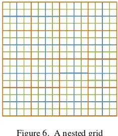
Both for aerial orhophotos and remote sensing images, the solution to the problems mentioned before resides in the use of a fixed and unique “nested grid” to produce, store, process, analyze, compare and serve orthoimages. A “nested grid” is a “space allocation schema” that assures completely coherent and consistent multiresolution coverage of the whole working area with orthoimages by organizing image footprints, pixel sizes and pixel positions at all pyramid levels. The term “nested” means that 2 by 2 images of each level of the pyramid are exactly contained in one image of the upper level, and also 2 x 2 pixels of each level are exactly contained in one pixel of the upper level, iteratively (Figure 6). This assures the alignment of pixels at all pyramid levels.
Figure 6. A nested grid
An example of a nested grid in use can be found in the “Australia National Nested Grid” (ANZLIC National Nested Grid Workgroup, 2012). The working area for this nested grid should be the whole Earth, or at least the biggest part of the inhabited areas, because local projections and grid schemas are no longer valid in present times.
In order to achieve these ambitious goals it is necessary to invert the traditional reasoning: instead of fixing a division in sheets and then try to aggregate them “upstairs” in the pyramid, we must start by one single rectangular image covering the whole Earth, end then begin to divide it in 2x2 parts, iteratively.
Any map projection that does not produce such a “global rectangle” is not suitable for building a nested grid, so it should be discarded for this purpose.
Two of the “rectangular” map projections are most used today, and should be considered: Geographic projection (Figure 7) and Mercator projection (Figure 8).
Neither Geographic nor Mercator projections are “equal area” but this is a minor problem compared with the advantages we are looking for.
Figure 7: Geographic projection covers the whole Earth with one rectangle. Source: Wikipedia
Figure 8: Mercator projection covers the biggest part of the inhabited areas with one rectangle. Source: Wikipedia
3. GEOGRAPHIC PROJECTION VERSUS MERCATOR PROJECTION
Geographic projection covers the whole Earth, but has a great disadvantage: it is not conformal so it changes the shape of all objects. For orthophotos it is very important to use a conformal projection in order to avoid strange appearance of common object and a “disagreeable perspective effect” in areas not near the equator. Even at medium latitudes (Figure 9) geographic projection makes rectangular buildings appear as rhomboidal, roundabouts appear as elliptical, etc. and produces an un-natural effect of “false perspective”. This problem becomes worse when going further to the North or to the South.
On the other hand Mercator projection does not cover the whole Earth, as a “cut” must be made at certain latitude to avoid infinite coordinates, but it covers the biggest part of the inhabited areas. And it is conformal, so it locally maintains the shapes of objects and they have a natural aspect at all latitudes (Figure 10).
The use of a conformal projection is also important in Remote Sensing, because it allows easy computation when dealing with directional effects such as BRDF, topographic shadows, etc. that are related with solar azimuth.
3.1 Web Mercator map projection
A particular implementation of Mercator projection has emerged as “de facto” standard in the last times for web mapping services: the “Spherical Mercator” or “Web Mercator” projection (EPSG:3857) used by Google Maps, Bing Maps, Yahoo Maps, Open Street Maps, ArcGIS Online and many
other geospatial data and API providers (ArcGis Online, 2009). It is associated to a Tiling Schema that is in fact a nested grid. Web Mercator is not perfectly conformal, because of the introduction of an “auxiliary” sphere to make computations easier, but it is “almost” conformal (the difference is very small) and looks conformal to the user.
Figure 9. Geographic projection 42º North
Figure 10. Mercator projection 42º North
The advantages of Web Mercator over other projections are described in (Schwartz, 2016) and (Daan 2012).
Web Mercator and the associated Tiling Schema are chosen for “WMTS Simple Profile” OGC standard (Open Geospatial Consortium, 2014). Web Mercator grid and tiling schema is fully documented and supported by many open source software libraries and a wide variety of commercial software.
3.2 The whole Earth in a single pixel
Web Mercator does another interesting and practical thing: It selects the “cut” latitudes in the exact places (85.05 degrees) so that the rectangle becomes square (Figure 11). We have now the whole Earth in one single square (or “in a single pixel”) that can be easily divided it in 2x2 recursively.
3.3 Pixel alignment at all pyramid levels
The tiles of Web Mercator Tiling Schema have no overlaps and have perfectly aligned borders at all levels. So pixels are aligned at all pyramid levels.
Figure 11. A square covers the whole working area in Web Mercator
4. THE QUADTREE STRUCTURE
As defined on the Wikipedia: “A quadtree is a tree data structure in which each internal node has exactly four children. Quadtrees are most often used to partition a two-dimensional space by recursively subdividing it into four quadrants or regions.” (Wikipedia 2016).
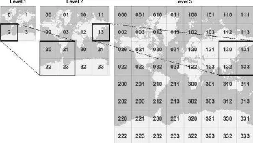
On Web Mercator tiling schema each tile is given (x,y) coordinates ranging from (0, 0) in the upper left to (2LOD-1, 2LOD-1) in the lower right. Figure 12 shows how tile 2 is divided in tiles 20, 21, 22 and 23, and tile 13 is divided in tiles 130, 131, 132 and 133.
Figure 12. Tile division and its nomenclature
As we can see in Table 13, the tiling schema starts in LOD 0 (Level of Detail 0) covering the whole working area (1) with one image of 256 x 256 pixels. Each time we increase zoom level (LOD), the pixel size divides by 2, and the number of pixels needed to cover the whole working area doubles. The square images (called “tiles”) inside each level are always 256x256 pixels. The size of 256x256 is chosen to optimize the visualization speed (minimize the time to fill the screen with tiles) for WMTS services. These tiles are sent, compressed in JPEG, by the WMTS Server in response to each demand of the web client.
4.1 Coherence with JPEG blocks
The size of 256 was also chosen because 256 is multiple of 8, and 8x8 is the “block” size of JPEG compression. This is very important in order to minimize image degradation, as it assures that 32x32 JPEG “blocks” fit exactly in each tile, thus avoiding
(1) The greatest part of inhabited areas (up to 85.05 degrees)
additional image degradation in possible subsequent mosaics due to the mix of “nonaligned” JPEG blocks.
All these sizes (8, 256…) are powers of 2 (2n) to allow “clean” pyramid building without border effects or surplus “orfan” pixels.
4.2 SuperTiles and BigTiles
256x256 tiles are way too small to be practical as “production units” (“sheets”) for uncompressed orthos, and even more for the compressed mosaics. So we propose to use as production units the same footprints of the Tiling Schema, but with a pixel size of other LOD.
For example: if we have LOD 14 pixel size and use LOD 8 footprints as “production units”, they would be 16,384 x 16,384 pixels. This produces images of about 1 Gbyte (with 4 bands in 8 bits per band), adequate for uncompressed images. For short we will call these images “SuperTiles”.
Given the pixel size of the orthoimagery we want to produce, we can choose the SuperTile size that best suits our application simply by selecting the adequate footprint between the different LOD.
Level of Detail (LOD)
World width and height
(pixels)
Pixel sizes at equator (m/pixel)
Map Scales (96 ppi screen) at
equator
0 256 156,543.0339 591,658,710.91
1 512 78,271.5170 295,829,355.45
2 1,024 39,135.7585 147,914,677.73
3 2,048 19,567.8792 73,957,338.86
4 4,096 9,783.9396 36,978,669.43
5 8,192 4,891.9698 18,489,334.72
6 16,384 2,445.9849 9,244,667.36
7 32,768 1,222.9925 4,622,333.68
8 65,536 611.4962 2,311,166.84
9 131,072 305.7481 1,155,583.42
10 262,144 152.8741 577,791.71
11 524,288 76.4370 288,895.85
12 1,048,576 38.2185 144,447.93
13 2,097,152 19.1093 72,223.96
14 4,194,304 9.5546 36,111.98
15 8,388,608 4.7773 18,055.99
16 16,777,216 2.3887 9,028.00
17 33,554,432 1.1943 4,514.00
18 67,108,864 0.5972 2,257.00
19 134,217,728 0.2986 1,128.50
20 268,435,456 0.1493 564.25
21 536,870,912 0.0746 282.12
22 1,073,741,824 0.0373 141.06
23 2,147,483,648 0.0187 70.53
Table 13. Pixel sizes and map scales at equator for Web Mercator Tiling Schema
In order to reduce the number of files and facilitate management and dissemination of data, we normally mosaic several orthophotos in one large compressed image file (e.g: in JPEG2000 format). For simplicity these compressed mosaics should be the composition of 4x4 or 8x8 uncompressed mosaics. For short we will call these mosaics “BigTiles”. The International Archives of the Photogrammetry, Remote Sensing and Spatial Information Sciences, Volume XLI-B2, 2016
5. TILED TIFF AS CONTAINER OF TILES
WMTS services require a huge number of tiles: hundreds of millions of individual “tiny” 256x256 JPEG files must be produced (either pre-cached or “on the fly”) in one or several “projections” (2) These tiles are very difficult to manage in current computing environments, because operating systems are not prepared for such a large number of files. Even listing them can be a challenge, and if an operator needs to check them looking for problems or errors (corrupted tiles, missing tiles, etc.) he will discover it is absolutely impossible with such a huge number of files. (It is like “looking for a needle in a haystack”). One possible solution is to store many tiny 256x256 tiles “inside” a bigger file. One way to do this is explained now:
5.1 Tiled TIFF
TIFF format has many options. One of them is called TiledTIFF. It was designed to allow quick access to any part of a big image without reading the whole file. TiledTIFF stores all the pixels in a tile together (while normal TIFF tiles store together all the pixels in a line)
When we generate a TiledTIFF we can choose the tile size. If we choose 256x256 tile size and the image size is a multiple of 256, the tiles we obtain inside the TiledTIFF are exactly the footprints and the pixel sizes Web Mercator Tiling Schema (of differents LOD as we saw before), we will end up with JPEG tiles inside the TiledTIFF that are exactly the same as the WMTS ready to be directly sent without the need to decompress and recompress them before sending,
With this approach we have two advantages at the same time: 1) We only compress once. So we save CPU time and preserve image quality
2) We do not have to generate millions of individual 256x256 JPEG files. So we don’t fall in the directory burden.
This approach has already been implemented by Mapserver opensource project (Bonfort, T. 2016).
5.3 All tiles pre-generated
We have to take into account that WMTS services performance advantage is based on the availability of “precached” tiles. Normally, we only “precache” 256x256 tiles until a certain LOD, because the work of generating them and the disk space to store JPEG files are so big, that it is not worth to pre-generate the LOD with smaller pixel sizes (the probability of being accessed is lower than for tiles of bigger pixel sizes). So normally, for this big LODs we wait until the first request to generate this tiles “on the fly”, and then cache them for future requests. So user sees a decrease in performance.
On the other hand, if we use TiledTIFF with JPEG compression as the format for compressed mosaics, all the tiles until the
(2) More rigorously: in one or several Spatial Reference Systems -SRS
native resolution are pregenerated, so there is no loss in performance at the biggest zoom levels.
5.4 Big TIFF
TIFF files have a limitation of 4 Gbytes, due to 32 bit offsets. BigTIFF unofficial standard uses 64-bit offsets thereby supporting files up to 18,000 petabytes. As BigTiles are usually bigger than 4 Gbytes, we must use BigTIFF format.
6. ADDITIONAL ISSUES
Some remaining issues should be addressed:
Issue 1: Mercator projection is not “equal area” nor “equidistant” as it has a different scale at each latitude. In other words, a fixed pixel size in the projection is in fact variable with latitude.
Issue 2: Pixel sizes (meters/pixel) in Table 13 are not integer, as we are used to.
Issue 3: Strange Map Scales. Map scales in Table 14 are not integer.
¿Can we find a solution for these issues?
6.1 Correct area and distances computation
For spatial analysis and reporting, where true area values are required, the solution is very simple: instead of counting pixels, take into account the real surface on the ground of each pixel (which is easily calculated using the “scale factor”). For visualization, the user has to get used to the fact that scale vary with latitude. This should not pose a problem: sailors have done it for centuries, because Marine Charts always use Mercator projection.
With respect to distances, we cannot directly measure correctly on Mercator, so a small rigorous calculation must be performed. This is not a problem in modern computing environments.
6.2 Secant Mercator Projection
There is a variant of Mercator projection that instead of a tangent cylinder uses a cylinder secant to the Earth in two parallels called “standard parallels” (Figure 14), where the scale is true (distances on the projection are equal to distances on the ground).
If we use this secant projection it is logical to use the two standard parallels as “reference” for pixel sizes. And we can calculate the latitude that produces integer pixel sizes in the table of LOD of WMTS Simple Profile tiling schema.
6.3 The advantages of integer pixel sizes
Integer pixel sizes are highly preferable to non-integer ones because operations with real number always have “rounding errors”. These errors accumulate when processing a large number of pixels, thus becoming a noticeable error in the form of visual “artifacts” such as “moiré”, missing lines, and other problems.
The latitude that produces integer pixel sizes happens to be 33.14489729º (see Table 15). So we could use a “Secant Mercator” projection with two standard parallels at 33.14489729º North and South (Figure 14). In these two The International Archives of the Photogrammetry, Remote Sensing and Spatial Information Sciences, Volume XLI-B2, 2016
parallels pixel sizes (measured in meters) are integer up to LOD 17. In centimeters, they are integer until LOD 19, in mm until LOD 20, and so on.
Figure 14. Secant Mercator map projection (from https://en.wikipedia.org/wiki/Mercator_projection)
6.4 Reference screen resolution of 254 ppi
The scale of an image displayed on a computer screen depends on the resolution (measured in pixels per inch –ppi-) of each screen. There is no obligation to use 96 ppi as a “reference” screen resolution (which produces ugly scale numbers even with “round” pixel sizes. As nowadays there exist a great variety of screen resolutions up to 400 ppi and more, we can choose one that produces “easy to remember” integer map scales. E.g.: 10 pixels/mm = 254 ppi. Then the LOD values look much better (Table 15) with integer pixel sizes and integer map scales, very easy to use.
7. APPLICATION TO DIGITAL ELEVATION MODELS
Digital Elevation Models and Orthoimages are mutually complementary for several reasons:
- DEMS are needed to orthorectify images once they have been captured by the sensor
- DEMS are also needed to perform some radiometric corrections such as topographic shadows corrections
- Orthoimages and DEMS can be combined to generate 3D (or 2.5 D) modeling
- etc.
So it is very important that we maximize the interoperability between both kinds of datasets. For this, it is imperative that they share a common grid and tiling schema.
Inspire Data Specification recognized this fact and for that reason included an Annex D describing this common grid both in Orthoimagery and in Elevation Data Themes. The problem is that, as we said before, the proposed Zoned Geographic Grid does not fulfill several of the requirements posed in this document for orthoimagey. Almost the same requirements are also applicable to Elevations, for analog reasons. This is the list of requirements, adapted to Elevation data:
1. Avoid the use of Map Projections with different zones. 2. Avoid repeated resampling. It is computing demanding and causes data degradation, so resampling should be avoided whenever possible. Ideally only one resampling should be performed during the whole process.
3. Height sampling points should be aligned at all levels of the pyramid
Table 15. Third and fourth columns show pixel sizes of Secant Web Mercator tiling schema with reference latitude 33.144º and
map scales on a 254 dpi screen at the same reference latitude.
For these reasons, the grid representation of DEMS should share the same nested grid as orthoimagery. There are only a few considerations that must be taken into account: Some algorithms use as input the Z coordinates of the center of orthoimagery pixels. E.g: orthorectification of an image using bicubic resampling, etc. Some other algorithms use as input the Z coordinates of the corners of orthoimagery pixels. E.g: topographic shadow correction, 2.5 D modeling by assigning color to the TIN triangles, orthorectification of an image using supersampling, etc. Should we measure and store the Z of the corners of the grid or the Z of the centers of the squares of the grid? Let’s take a common situation: suppose we have a 5m grid spacing DEM and we want to generate a 25 cm pixel size aerial orthophoto. We find these facts:
7.1 Sampling distance
If we look to the green columns of Table 15, the first thing we see is that 5m is not a pixel size in the table, because all pixel sizes in the table are powers of 2 in these green columns. So if we want a complete coherence between ortho and DEM we should use a 4m DEM, instead of a 5m DEM. So the first advice is: choose a DEM sampling that is one of the pixel sizes of the nested grid.
7.2 Heigh interpolation
The second thing we see is that sample spacing of the DEM is much bigger than ortho pixel size: 4m versus 25cm is 16 times bigger. So if we need the Z of the centers of the orthoimage pixels as well as if we need the Z of the corners of the pixels, we are obliged to interpolate in both cases. The interpolation The International Archives of the Photogrammetry, Remote Sensing and Spatial Information Sciences, Volume XLI-B2, 2016
seems easier to perform starting with the corners of the pixels, but not anything very important.
7.3 Pyramid consistency
If we measure and store the Z of the center of the image pixels in LOD n (Figure 16 left) in order to generate LOD n-1 we have to resample the heights (Figure 16 right) because there is no positional coincidence of the centers.
Resampling the heights produces a “degradation” of height values (loss of accuracy and appearance of artifacts) in the same way as a resampling an image produces a degradation of radiometric values. This need to resample the heights happens in all the changes of LOD, so there is a cumulative degradation of height values when we go up the pyramid of LOD. On the other hand, if we have the Z of the corners of the pixels in LOD = n (Figure 17 left), in order to generate LOD = n-1 we don’t need to interpolate (Figure 17 right) because there is positional coincidence of the corners.
Figure 16. Left: in black, centers of blue pixels (LOD=n). Right: in green, centers of red pixels (LOD=n-1)
Figure 17. Left: in black, corners of blue pixels (LOD=n). Right: in green, corners of red pixels (LOD=n-1)
For this reason, and also because it seems a simpler schema easier to understand, and so less likely to produce mistakes, we recommend the second option: we should measure and store in the DEMs the corners of the nested grid, not the centers.
8. APPLICATION TO RASTER MAPS
Raster maps can suffer the same problems than orthoimages and DEMS: loss of processing power, degradation of image quality, visual artifacts (due to black wedges and other problems), etc. These problems cause great inefficiencies in production, dissemination through web services and use from light web clients or desktop GIS programs. Also, they suffer the same problem with the big number of JPEG tiles that must be generated (either “precached” or on the fly) for a WMTS service.
We have to take into account that WMTS services performance advantage is based in the availability of “precached” tiles, with the pixels in the exact places. So if we need to overlay orthoimages, DEMs and raster maps in the same viewer, we will attain top visual performance only if we use the same map
projection, pixel sizes and pixels positions for all layers being displayed, avoiding the use of any resampling. For these reasons, our recommendation is to use for raster maps production and dissemination the same nested grid than for orthoimagery and DEMS. In this way, a perfect coherence would be achieved for all these types of data.
9. CONCLUSSIONS
We have shown that usual workflows for production, archiving, dissemination and use of raster geographic data pose big interoperability problems. Web Mercator map projection and associated tiling schema as a nested grid that would help to ease the solution to most of them. The adoption of this nested grid by National Mapping and Cadastral Agencies and Space Agencies would greatly facilitate the interoperability between raster data all over the world.
ACKNOWLEDGEMENTS
This work was performed with the financing of Spanish “Ministerio de Economía y Competitividad” under the “Programa Estatal de Fomento de la Investigación Científica y Técnica de Excelencia” (Ingenio L2 coordinated Project).
REFERENCES
ANZLIC National Nested Grid Workgroup, 2012, National Nested Grid Specification Guideline
http://www.anzlic.gov.au/sites/default/files/files/Guide_master_ NNG_GSF_20120808.pdf
Wikipedia contributors, "List of map projections", Wikipedia, (accessed April 16, 2016)
https://en.wikipedia.org/w/index.php?title=List_of_map_project ions&oldid=715022714
Wikipedia contributors, "Quadtree", Wikipedia (accessed April 16, 2016) https://en.wikipedia.org/wiki/Quadtree
Schwart, J., 2016. Bing Maps Tile System. MSDN Library. https://msdn.microsoft.com/en-us/library/bb259689.aspx
Daan, Why Mercator for the Web? Isn’t the Mercator bad? Mapthematics Forums (accessed April 16, 2016)
http://www.mapthematics.com/forums/viewtopic.php?f=8&t=25 1
ArcGIS Server Development Team, 2009. ArcGIS Online moving to Google / Bing tiling scheme: What does this mean for you?
http://blogs.esri.com/esri/arcgis/2009/11/20/arcgis-online- moving-to-google-bing-tiling-scheme-what-does-this-mean-for-you/
Open Geospatial Consortium, 2014, Web Map Tile Service (WMTS) Simple Profile. OGC®
http://docs.opengeospatial.org/is/13-082r2/13-082r2.html
Bonfort, T. Cache Types, Map Server Open source Web Mapping (accessed April 16, 2016)
http://mapserver.org/es/mapcache/caches.html#geo-tiff-caches) The International Archives of the Photogrammetry, Remote Sensing and Spatial Information Sciences, Volume XLI-B2, 2016