PERFORMANCE EVALUATION OF sUAS EQUIPPED WITH VELODYNE HDL-32E
LiDAR SENSOR
G. Jozkow a, *, P. Wieczorek a, M. Karpina a, A. Walicka a, A. Borkowski a
a Institute of Geodesy and Geoinformatics, Wroclaw University of Environmental and Life Sciences, Poland – (grzegorz.jozkow, mateusz.karpina, agata.walicka, andrzej.borkowski)@igig.up.wroc.pl, [email protected]
Commission I, ICWG I/II
KEY WORDS: UAS, LiDAR, Velodyne, performance evaluation
ABSTRACT:
The Velodyne HDL-32E laser scanner is used more frequently as main mapping sensor in small commercial UASs. However, there is still little information about the actual accuracy of point clouds collected with such UASs. This work evaluates empirically the accuracy of the point cloud collected with such UAS. Accuracy assessment was conducted in four aspects: impact of sensors on theoretical point cloud accuracy, trajectory reconstruction quality, and internal and absolute point cloud accuracies. Theoretical point cloud accuracy was evaluated by calculating 3D position error knowing errors of used sensors. The quality of trajectory reconstruction was assessed by comparing position and attitude differences from forward and reverse EKF solution. Internal and absolute accuracies were evaluated by fitting planes to 8 point cloud samples extracted for planar surfaces. In addition, the absolute accuracy was also determined by calculating point 3D distances between LiDAR UAS and reference TLS point clouds. Test data consisted of point clouds collected in two separate flights performed over the same area. Executed experiments showed that in tested UAS, the trajectory reconstruction, especially attitude, has significant impact on point cloud accuracy. Estimated absolute accuracy of point clouds collected during both test flights was better than 10 cm, thus investigated UAS fits mapping-grade category.
1. INTRODUCTION
Although typical UAS (Unmanned Aerial System) used for mapping purposes is equipped with RGB camera, LiDAR (Light Detection and Ranging) sensors are more and more often mounted, even on electrically powered sUAS (small UAS). A lot of them base on one of Velodyne sensors: HDL-32E or VLP-16 (Puck), because these scanners are relatively lightweight, can be purchased for a reasonable price, and are successfully used in mobile mapping applications (Hauser et al., 2016). Laser scanners are usually mounted on multirotor UAVs (Unmanned Aerial Vehicles) since these platforms can handle heavier payload, however, there are also implementations with gas propelled fixed-wing platforms (Khan et al., 2017). Unfortunately, multirotor platforms offer less stable flight than fixed-wing UAVs that negatively impacts the quality of collected point clouds. Beside the laser scanner, LiDAR UAS used for large scale mapping must be equipped also with tactical-grade IMU (Inertial Measurement Unit) and geodetic-grade GNSS (Global Navigation Satellite System) sensors, because direct georeferencing capability is required (Grejner-Brzezinska et al., 2015). Typically, MEMS (Micro Electro Mechanical System) IMUs and miniaturized dual-frequency GNSS receivers and antennas are used.
Despite the fact that commercial LiDAR UASs equipped with relatively inexpensive Velodyne sensors are available on the market, there is still little information about the performance of such systems. Recent studies analyzed theoretical accuracy of the data derived by lightweight LiDAR UASs (Pilarska et al., 2016), provided initial results indicating issues with accurate point cloud georeferencing (Jozkow et al., 2016), or just mentioned obtained accuracy without detailed analysis (Sankey et al., 2017). Theoretical analysis of the point cloud accuracy showed that
* Corresponding author
lightweight UAS equipped with Velodyne scanner can achieve mapping-grade accuracy (Pilarska et al., 2016), but reported in practice accuracy was much lower and equal to about 1.3 and 2.3 m for horizontal, and vertical components, respectively (Sankey et al., 2017). In contrast, UASs equipped with high-end laser scanner and navigation sensors can achieve accuracy comparable to airborne LiDAR (Wieser et al., 2016) that qualifies them to survey-grade category. Note that accuracy categories mentioned in this work are the same as used by Hauser et al. (2016) and mean 3D point accuracy up to 5 cm, and 5-20 cm, at one sigma, for survey-grade, and mapping-grade categories, respectively.
This work aims on empirical accuracy assessment of LiDAR UAS data collected by Velodyne HDL-32E laser scanner mounted on hexacopter platform. The evaluation was executed in terms of 3D point absolute accuracy that determines system category. Absolute accuracy was evaluated by comparing UAS point cloud with the reference TLS (Terrestrial Laser Scanning) point cloud of much higher accuracy. In addition internal accuracy of UAS point cloud was evaluated, and the analysis of trajectory reconstruction results was performed as the most significant factor that impacts point cloud absolute accuracy.
2. MATERIALS AND METHODS
2.1 Equipment
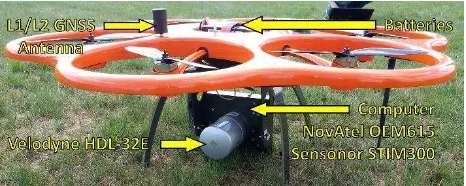
Test platform used in the investigation was Aibot X6 that is hexacopter type I of around 1 m diameter and maximal take-off weight 6.6 kg, thus it qualifies to sUAS category. It is powered by 2 5-cell Li-Po batteries with the capacity of 5 Ah each, that allows to fly around 6-8 minutes in the LiDAR configuration. The system is equipped with Velodyne HDL-32E laser scanner, The International Archives of the Photogrammetry, Remote Sensing and Spatial Information Sciences, Volume XLII-2/W6, 2017
NovAtel OEM615 GNSS receiver and dual-frequency GNSS antenna, and Sensonor STIM300 IMU. According to specification, the accuracy (one sigma) of Velodyne is 2 cm at 25 m. The performance of navigational sensors (GNSS and IMU) is specified by the manufacturer as the accuracy of trajectory position and attitude that is post processed by integrating GNSS (from base and rover stations) and IMU observations (Table 1). Note that given accuracies refer to ideal test conditions for ground vehicle data. Because tested UAS uses only one geodetic grade GNSS antenna, therefore it requires kinematic alignment of the azimuth.
Position accuracy [m] RMS Horizontal 0.01 Vertical 0.02
Attitude accuracy [°] RMS Pitch Roll 0.006 0.006 Yaw 0.019 Table 1. Manufacturer specified performance of navigational
sensors used in tested UAS (description in the text).
All three sensors (laser scanner, GNSS receiver, and IMU) together with a small computer that uses Windows operating system are assembled together and fixed to the gimbal (Figure 1). Test UAS is a multi-purpose system since it can be equipped with different 2-axis gimbal that is suitable for variety of cameras, but only LiDAR configuration was used to collect data for this investigation. Although this UAS was manufactured and calibrated by a professional company, it is custom and unique construction.
Figure 1. UAS used to collect LiDAR data.
Additional equipment used to collect data for this investigation consisted of two geodetic-grade ground GNSS base stations placed on a site. One station was treated as a backup, though GNSS data from stations was investigated in this study. Reference point cloud was collected with Leica ScanStation P20 terrestrial laser scanner.
2.2 Test flights and data
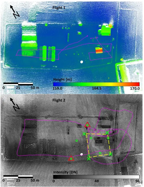
LiDAR UAS data used in this investigation was collected during two separate flights (referred here as Flight 1 and Flight 2)
executed over the same site containing mostly man-made objects (the largest one was a 2-storey building), and low and medium vegetation (Figure 2). The Flight 1 was executed in autonomous mode, i.e. the flight was performed automatically according to prepared flight plan except take-off and landing. Note that UAV during autonomous flight may hover, do sharp turns or even fly backwards. Such type of movements may cause issues during GNSS and IMU data integration. The Flight 2 was executed manually by UAV operator. This mode was selected to keep UAV flying forward and avoid hexacopter hovering. Unfortunately, during manual mode it was practically impossible to flight according to flight plan lines. For that reason, scanner FOV (Field of View) was not limited to a certain angle. Note that position accuracy of points collected at large incidence angles is usually lower. Both test flights were executed at the altitude equal to 25 m AGL (Above Ground Level) and with ground speed equal to 4 m/s. During manual flight, small variations to these values were unavoidable.
Beside the on-board LiDAR and navigational data, also the GNSS data from 3 base stations was acquired. In addition to 2 user stations placed on the site (Figure 2), the data from the EPN (EUREF Permanent Network) station was downloaded and investigated in trajectory reconstruction. Used EPN station was only about 5.5 km away from test site. More than one and placed at different distances base stations allowed to compare UAS trajectories obtained with different configurations of GNSS network.
The reference TLS data was collected from 4 stations (Figure 2). Theirs location was selected to minimize occlusions in test area (Figure 2) – the goal was to scan each part of building from two stations. To maximize the quality of collected TLS data, black and white targets were used for point cloud co-registration and georeferencing. The co-registration was executed based on 6 targets (Figure 2), where 4 of them got accurate geodetic coordinates and were subsequently used in TLS data georeferencing.
The basic statistics of collected point clouds are given in Table 2. Point clouds collected during both flights and UAV trajectories are visualized in Figure 2.
Survey Flight 1 Flight 2 TLS
Number of points 72.7M 134.6M 37.7M Point density [points/m2] 5K 14K 60K Table 2. Approximated number of points collected at test site
and average point density in test area. The International Archives of the Photogrammetry, Remote Sensing and Spatial Information Sciences, Volume XLII-2/W6, 2017
Figure 2. Point clouds collected during test flights: Flight 1 on top (heights coded in colors), Flight 2 on bottom (intensities coded in grays). Meaning of symbols and colors: red triangles – GNSS base stations, purple lines – actual UAV trajectories, green x – TLS stations, green circles – TLS targets used for co-registration and georeferencing, yellow border – test area containing reference TLS
data.
2.3 Data processing
Collected raw data was processed according to typical workflow of kinematic LiDAR data processing. In general, this processing aims on transforming Cartesian coordinates of each point collected at time � from scanner coordinate system (s-frame) to ECEF (Earth-Centered, Earth-Fixed) coordinate system (e-frame). Obviously, Cartesian coordinates in s-frame are calculated for each point based on measured range, angles, and known scanner calibration parameters. Also coordinates given in e-frame are further transformed to other (e.g. national) coordinate system by applying appropriate projection and geoid model. The transformation from s-frame to e-frame is executed in a few steps that include results of GNSS and IMU data integration and intra-sensor calibration parameters. This transformation is executed according to direct georeferencing equation:
� � =
�� � + ��� � ∙ ��� � ∙ ��+ ���∙ � � (1)
where � � – Cartesian coordinates of point in s-frame �� – position of s-frame origin in IMU coordinate system (b-frame), i.e. scanner-to-IMU lever-arm offset
���= ��� �, �, – rotation matrix describing the
rotation from s-frame to b-frame, i.e. bore-sight alignment that is parameterized through three Euler angles �, �,
��� � = ���(� � , � � , � ) – rotation matrix
describing the rotation from b-frame to n-frame; it depends on the roll �, pitch �, and yaw angles
��� � = ���( � , � � )– rotation matrix describing the rotation from navigational topocentric coordinate system (n-frame) to e-frame; it depends on the executed using commercial software. Results of trajectory reconstruction consisted of sets of IMU (b-frame origin) positions in e-frame �� � , and IMU attitudes (�, �, and angles) in n-frame used to calculate rotation matrix ��� � . In the second step, coordinates of points given in s-frame � � were transformed to e-frame coordinates � � according to Eq. 1. Because the trajectory was reconstructed for different time stamps � and with lower rate than for points, IMU position and attitude that matched point time stamps were interpolated using B-splines. The position of IMU in e-frame �� � was also used to calculate longitude and latitude, and consequently, rotation matrix ���. Note that scanner-to-IMU lever-arm offset �� and bore-sight alignment used to calculate rotation matrix ��� were known from manufacturer provided calibration.
The point cloud obtained in e-frame was then transformed to more useful national coordinate system and pre-processed in order to remove gross errors (i.e. low and high points).
Reference TLS data collected from 4 stations was co-registered using 6 targets, and then georeferenced based on 4 targets that had coordinates specified in the same national coordinate system. Note that only 2 targets were necessary for co-registration and georeferencing, because the scanner was levelled at each station. The co-registration, and the georeferencing resulted in mean
absolute errors equal to 3 and 9 mm, respectively. It means that reference data should be more accurate than UAS point cloud, therefore can be used as a reference.
2.4 Performance evaluation methodology
The performance evaluation of described UAS was executed in this work in four aspects:
Impact of sensor errors on point cloud accuracy in ideal conditions
Trajectory reconstruction quality as the sensor dependent factor affecting point cloud accuracy Point cloud internal accuracy
Point cloud absolute accuracy
Knowing the performance of navigational sensors (Table 1) and laser scanner, theoretical accuracy of collected points can be evaluated by applying covariance propagation rule to Eq. 1. Obviously, given parameters refer to laboratory (ideal) conditions, but they allow to estimate expected magnitude of point cloud accuracy.
The analysis of trajectory reconstruction quality was executed by calculating differences (separations) of trajectory position and attitude obtained from forward and reverse EKF solutions. Values of these separations were treated in this study as accuracy measures.
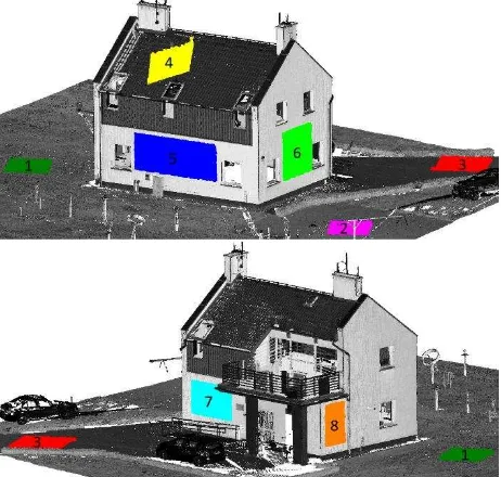
Point cloud internal accuracy was evaluated based on 8 point cloud samples extracted for at least 1 m2 surfaces belonging to planar objects. There were selected: 3 horizontal ground surfaces, 1 oblique surface of building roof, and 4 vertical surfaces of building walls (Figure 3). The plane was fitted into each sample cloud using MSAC (M-estimator SAmple Consensus) algorithm (Torr and Zisserman, 2000). This algorithm assures that fitted planes are robust to outlier points (e.g. created by multipath reflections) that were not removed during point cloud pre-processing. After fitting planes to each point cloud sample, the distances from points to fitted planes were calculated. These distances were treated as residuals and were used to calculate RMSE (Root Mean Square Error) that describes point cloud internal accuracy.
Figure 3. Location of 8 point cloud samples (color patches) used in accuracy evaluation, and reference TLS point cloud (gray). The International Archives of the Photogrammetry, Remote Sensing and Spatial Information Sciences, Volume XLII-2/W6, 2017
It should be emphasized that internal accuracy estimated in this manner is affected by actual planarity of selected surfaces, theirs roughness, and also point cloud direct georeferencing process. It was observed that each sample plane was scanned from 2 to 11 UAV passes (trajectory sections), thus RMSE calculated from all passes was affected also by trajectory reconstruction, especially if the sample surface was scanned at the beginning and at the end of the flight. Note that the analysis was executed on entire point cloud, collected also during manual flight, and UAV take-off and landing, therefore the strip adjustment was not applied. To minimize the impact of point cloud georeferencing on internal accuracy, plane fitting and residual calculation was executed also separately for single UAV passes.
Point cloud absolute accuracy was estimated using two methods. The first method was similar to described above method for internal accuracy assessment, however, reference planes were estimated from accurate TLS data. The second method also used distances as residuals, but they were calculated for entire point cloud included in test area. These distances were calculated between UAS points and theirs nearest neighbors from TLS point cloud. High density of reference point cloud should not cause larger residuals, and consequently RMSE. Obviously, occluded areas in any of the point cloud were excluded from the test area. Note that UAS and TLS points belonging to the same surface were created from laser beams of significantly different incidence angles, therefore they have different characteristic, especially for rough surfaces, such as lawn. However, this issue has rather minor impact and should not significantly reduce calculated absolute accuracy of UAS point cloud.
3. RESULTS AND DISCUSSION
3.1 Impact of sensors on point cloud accuracy
The impact of sensors was evaluated by calculating distribution of 3D position error in single scanning swath created on a flat terrain by one revolution of Velodyne scanner in 120° field of view (from –60° to +60° from nadir direction) caused by sensor errors. Known values, such as lever-arm offset, bore-sight alignment and flying height (25 m) were used in this calculation. Unknown values, e.g. accuracies of lever-arm offset and bore-sight as well as roll, pitch, and yaw angles were set to zero. It was also assumed that UAV is not moving and incidence angle has insignificant impact on 3D position accuracy. Obtained theoretical point 3D position accuracy with respect to point location in the swath is shown in Figure 4. Note that Velodyne HDL-32E collects points arranged in 32 scanning lines, but continuous swath was shown only for visualization purposes.
Figure 4. Distribution of point 3D position error in Velodyne HDL-32E swath caused by typical errors of used scanner and navigational sensors (25 m flying height over flat terrain).
Point cloud accuracy possible to achieve with tested UAS at 25 m flying height and in ideal flying conditions is equal to about 30 mm in the nadir direction, to about 35 mm in swath corners (Figure 4). It means that this UAS in optimal conditions may be suitable for survey-grade applications, however, it should be expected that real point cloud will have mapping-grade accuracy, because other errors were not included in error propagation.
3.2 Trajectory reconstruction
The analysis of navigational data used for trajectory reconstruction showed its completeness and good quality. The number of visible GPS and GLONASS satellites was at least 13. Regardless of the GNSS base station configuration (single user station on a site, farther EPN station, 2 stations, or 3 stations), the same trajectory was computed – differences in position and attitude were insignificant.
The analysis of position separation (Figure 5) showed that it is close to manufacturer specified accuracy (Table 1) equal to 1 and 2 cm for horizontal and vertical components, respectively. Only three small sections of Flight 2 trajectory showed larger horizontal separations up to 14 cm (Figure 5).
Figure 5. UAV position differences calculated between forward and reverse EKF solution.
The analysis of attitude separation (Figure 6) showed higher divergences with respect to manufacturer specification (Table 1). In the Flight 1, differences to roll/pitch and yaw angles were in absolute terms up to 0.03° and 0.15°, respectively. In the Flight 2, differences were much higher and for major part of the flight were up to about 0.15° and 0.5° (in absolute terms), for roll/pitch and yaw angles, respectively. Lower than specified attitude accuracy (Table 1) may be explained by flight dynamics. The movement of multirotor platform is strongly affected by wind and significantly less smoother than movement of ground vehicle. Lower accuracy of Flight 2 attitude, though the flight was executed manually, may be attributed to worse kinematic alignment of initial attitude, especially azimuth, and will likely decrease the accuracy of the point cloud.
Figure 6. UAV position differences calculated between forward and reverse EKF solution.
3.3 Point cloud internal accuracy
Internal accuracy was evaluated separately for both flights in two variants. In the first variant, RMSE was calculated based on residuals to 8 planes fitted to point cloud samples. In the second variant, residuals were measured to planes fitted into part of the point cloud samples collected during single pass of UAV. Obtained accuracies are shown in Table 3.
Variant Flight 1 Flight 2 Reference TLS data
1 61 73
5
2 50 68
Table 3. Point cloud internal accuracy (RMSE [mm]) evaluated in two variants (description in the text).
Results show that slightly lower accuracy was obtained for Flight 2. Differences occur also between methods (variants) of internal accuracy estimation. For example, sample surface no. 8 (Figure 3) was scanned during Flight 1 in 5 UAV passes (Figure 7) resulting in the highest RMSE calculated for single surface according to first variant, and equal to 122 mm. However, point clouds collected for this surface in single pass were very consistent (Figure 7), thus RMSE calculated for this sample surface but in second variant resulted in RMSE equal to only 20 mm. Different position and orientation of the point cloud obtained for this sample in different passes was caused by georeferencing errors not internal accuracy of the data. For that reason, RMSE calculated in the second variant is more reliable measure of internal accuracy of the point cloud.
Figure 7. Side view on point clouds collected for sample surface no. 8 during Flight 1 (colors indicate points collected in separate UAV passes), and by terrestrial laser scanner (black points).
Because internal accuracy calculated in both variants could be affected by surface roughness, and actual geometry of sample surface that is not strictly the plane, Table 3. includes also RMSE of fitting the plane into reference TLS data. Obtained RMSE equal to only 5 mm shows that sample surfaces are close to planes. Note that used terrestrial laser scanner collects points with 3D accuracy equal to 3 mm at 50 m range. The largest RMSE for reference data was achieved for the sample surface no. 1 (Figure 3) and was equal to 14 mm. This surface was the freshly mowed lawn and was the most rough among test samples.
3.4 Point cloud absolute accuracy
Both methods of absolute accuracy evaluation resulted in similar RMSE (Table 4). For both flights, calculated point cloud absolute error is lower than 10 cm. It means that investigated UAS is able to provide data with mapping-grade accuracy. However, point cloud accuracy collected during Flight 2 is lower than for Flight 1. Lower accuracy of the second data set can be explained by mentioned earlier lower accuracy of reconstructed trajectory, (especially attitude), and lower internal accuracy. Analysis of distances between UAS and TLS point clouds (Figure 8) also proves lower accuracy of point cloud collected during Flight 2 – the number of larger distances is higher than for point cloud collected during Flight 1.
Method Flight 1 Flight 2
Distances to reference plane 75 92 Distances to reference point cloud 64 91 Table 4. LiDAR UAS point cloud absolute accuracy
(RMSE [mm]) evaluated with 2 different methods.
Figure 8. 3D distances between LiDAR UAS and reference TLS points. Occluded areas were removed from the analysis.
4. CONCLUSIONS
This work evaluated the accuracy of the data collected with Velodyne HDL-32E laser scanner mounted on multirotor UAV. The evaluation focused on determining the absolute accuracy of the point cloud based on the reference TLS data. In addition, assessment of point cloud internal accuracy, impact of sensor errors and trajectory reconstruction quality were also investigated. The latter one factor was indicated as the most significant that affects the accuracy. Obtained results showed that investigated UAS equipped with Velodyne HDL-32E laser scanner can provide point clouds of the absolute 3D position accuracy not worse than 10 cm, thus it suits mapping-grade applications. The accuracy could be possibly improved by applying scan adjustment to correct UAV position, and especially, the attitude. This task will be investigated in the future.
REFERENCES
Jozkow, G., Toth, C., Grejner-Brzezinska, D., 2016. UAS topographic mapping with Velodyne LiDAR sensor. In: ISPRS Annals of the Photogrammetry, Remote Sensing and Spatial Information Sciences, Vol. III-1, pp. 201-208.
Grejner-Brzezinska, D., Toth, C., Jozkow, G., 2015. On Sensor Georeferencing and Point Cloud Generation with sUAS. Proc. Of the ION 2015 Pacific PNT Meeting, April 20-23, Honolulu, USA, pp. 839-848.
Hauser, D., Glennie, C., Brooks, B., 2016. Calibration and accuracy analysis of a low-cost mapping-grade mobile laser scanning system. Journal of Surveying Engineering, 142(4), pp. 04016011.
Pilarska, M., Ostrowski, W., Bakuła, K., Górski, K. Kurczyński, Z., 2016. The potential of light laser scanners developed for unmanned aerial vehicles – the review and accuracy. International Archives of the Photogrammetry, Remote Sensing and Spatial Information Sciences, XLII-2/W2, pp. 87-95.
Khan, S., Aragão, L., Iriarte, J., 2017. A UAV–lidar system to map Amazonian rainforest and its ancient landscape transformations. International Journal of Remote Sensing, 38(8-10), pp. 2313-2330.
Sankey, T., Donager, J., McVay, J., Sankey, J.B., 2017. UAV lidar and hyperspectral fusion for forest monitoring in the southwestern USA. Remote Sensing of Environment, 195, pp. 30-43.
Wieser, M., Hollaus, M., Mandlburger, G., Glira, P., Pfeifer, N., 2016. ULS LiDAR supported analyses of laser beam penetration from different ALS systems into vegetation. ISPRS Annals of the Photogrammetry, Remote Sensing & Spatial Information Sciences, III-3, pp. 233-239.
Torr, P.H., Zisserman, A., 2000. MLESAC: A new robust estimator with application to estimating image geometry. Computer Vision and Image Understanding, 78(1), pp. 138-156.

![Table 4. LiDAR UAS point cloud absolute accuracy (RMSE [mm]) evaluated with 2 different methods](https://thumb-ap.123doks.com/thumbv2/123dok/3304566.1405152/6.595.305.539.138.410/table-lidar-point-absolute-accuracy-evaluated-different-methods.webp)
