A fast learning algorithm for deep belief nets
∗Geoffrey E. Hinton
and
Simon Osindero
Department of Computer Science University of Toronto 10 Kings College Road
Toronto, Canada M5S 3G4 {hinton, osindero}@cs.toronto.edu
Yee-Whye Teh
Department of Computer Science National University of Singapore 3 Science Drive 3, Singapore, 117543Abstract
We show how to use “complementary priors” to eliminate the explaining away effects that make inference difficult in densely-connected belief nets that have many hidden layers. Using com-plementary priors, we derive a fast, greedy algo-rithm that can learn deep, directed belief networks one layer at a time, provided the top two lay-ers form an undirected associative memory. The fast, greedy algorithm is used to initialize a slower learning procedure that fine-tunes the weights us-ing a contrastive version of the wake-sleep algo-rithm. After fine-tuning, a network with three hidden layers forms a very good generative model of the joint distribution of handwritten digit im-ages and their labels. This generative model gives better digit classification than the best discrimi-native learning algorithms. The low-dimensional manifolds on which the digits lie are modelled by long ravines in the free-energy landscape of the top-level associative memory and it is easy to ex-plore these ravines by using the directed connec-tions to display what the associative memory has in mind.
1
Introduction
Learning is difficult in densely-connected, directed belief nets that have many hidden layers because it is difficult to infer the conditional distribution of the hidden activities when given a data vector. Variational methods use simple approximations to the true conditional distribution, but the approximations may be poor, especially at the deepest hidden layer where the prior assumes independence. Also, variational learning still requires all of the parameters to be learned together and makes the learning time scale poorly as the number of param-eters increases.
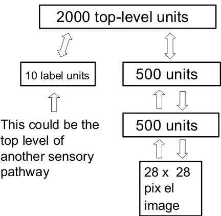
We describe a model in which the top two hidden layers form anundirectedassociative memory (see figure 1) and the
∗To appear in Neural Computation 2006
remaining hidden layers form a directed acyclic graph that converts the representations in the associative memory into observable variables such as the pixels of an image. This hy-brid model has some attractive features:
1. There is a fast, greedy learning algorithm that can find a fairly good set of parameters quickly, even in deep networks with millions of parameters and many hidden layers.
2. The learning algorithm is unsupervised but can be ap-plied to labeled data by learning a model that generates both the label and the data.
3. There is a fine-tuning algorithm that learns an excel-lent generative model which outperforms discrimina-tive methods on the MNIST database of hand-written digits.
4. The generative model makes it easy to interpret the dis-tributed representations in the deep hidden layers. 5. The inference required for forming a percept is both fast
and accurate.
6. The learning algorithm is local: adjustments to a synapse strength depend only on the states of the pre-synaptic and post-pre-synaptic neuron.
7. The communication is simple: neurons only need to communicate their stochastic binary states.
Section 2 introduces the idea of a “complementary” prior which exactly cancels the “explaining away” phenomenon that makes inference difficult in directed models. An exam-ple of a directed belief network with comexam-plementary priors is presented. Section 3 shows the equivalence between re-stricted Boltzmann machines and infinite directed networks with tied weights.
2000 top-level units
500 units
500 units
28 x 28
pix el
image
10 label units
This could be the
top level of
another sensory
pathway
Figure 1: The network used to model the joint distribution of digit images and digit labels. In this paper, each training case consists of an image and an explicit class label, but work in progress has shown that the same learning algorithm can be used if the “labels” are replaced by a multilayer pathway whose inputs are spectrograms from multiple different speak-ers saying isolated digits. The network then learns to generate pairs that consist of an image and a spectrogram of the same digit class.
is used to construct deep directed nets is itself an undirected graphical model.
Section 5 shows how the weights produced by the fast greedy algorithm can be fine-tuned using the “up-down” gorithm. This is a contrastive version of the wake-sleep al-gorithm Hinton et al. (1995) that does not suffer from the “mode-averaging” problems that can cause the wake-sleep al-gorithm to learn poor recognition weights.
Section 6 shows the pattern recognition performance of a network with three hidden layers and about 1.7 million weights on the MNIST set of handwritten digits. When no knowledge of geometry is provided and there is no special preprocessing, the generalization performance of the network is 1.25% errors on the10,000digit official test set. This beats the 1.5% achieved by the best back-propagation nets when they are not hand-crafted for this particular application. It is also slightly better than the 1.4% errors reported by Decoste and Schoelkopf (2002) for support vector machines on the same task.
Finally, section 7 shows what happens in the mind of the network when it is running without being constrained by vi-sual input. The network has a full generative model, so it is easy to look into its mind – we simply generate an image from its high-level representations.
Throughout the paper, we will consider nets composed of
Figure 2: A simple logistic belief net containing two inde-pendent, rare causes that become highly anti-correlated when we observe the house jumping. The bias of−10on the earth-quake node means that, in the absence of any observation, this node ise10times more likely to be off than on. If the
earth-quake node is on and the truck node is off, the jump node has a total input of0which means that it has an even chance of being on. This is a much better explanation of the observation that the house jumped than the odds ofe−20 which apply if
neither of the hidden causes is active. But it is wasteful to turn on both hidden causes to explain the observation because the probability of them both happening ise−10×e−10=e−20.
When the earthquake node is turned on it “explains away” the evidence for the truck node.
stochastic binary variables but the ideas can be generalized to other models in which the log probability of a variable is an additive function of the states of its directly-connected neigh-bours (see Appendix A for details).
2
Complementary priors
The phenomenon of explaining away (illustrated in figure 2) makes inference difficult in directed belief nets. In densely connected networks, the posterior distribution over the hid-den variables is intractable except in a few special cases such as mixture models or linear models with additive Gaussian noise. Markov Chain Monte Carlo methods (Neal, 1992) can be used to sample from the posterior, but they are typically very time consuming. Variational methods (Neal and Hinton, 1998) approximate the true posterior with a more tractable distribution and they can be used to improve a lower bound on the log probability of the training data. It is comforting that learning is guaranteed to improve a variational bound even when the inference of the hidden states is done incorrectly, but it would be much better to find a way of eliminating ex-plaining away altogether, even in models whose hidden vari-ables have highly correlated effects on the visible varivari-ables. It is widely assumed that this is impossible.
probability of turning on unitiis a logistic function of the states of its immediate ancestors,j, and of the weights,wij,
on the directed connections from the ancestors:
p(si= 1) =
1
1 + exp(−bi−Pjsjwij)
(1)
where bi is the bias of unit i. If a logistic belief net only
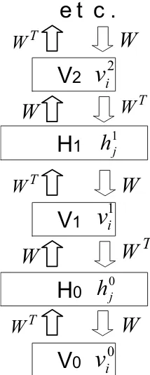
has one hidden layer, the prior distribution over the hidden variables is factorial because their binary states are chosen independently when the model is used to generate data. The non-independence in the posterior distribution is created by the likelihood term coming from the data. Perhaps we could eliminate explaining away in the first hidden layer by using extra hidden layers to create a “complementary” prior that has exactly the opposite correlations to those in the likeli-hood term. Then, when the likelilikeli-hood term is multiplied by the prior, we will get a posterior that is exactly factorial. It is not at all obvious that complementary priors exist, but figure 3 shows a simple example of an infinite logistic belief net with tied weights in which the priors are complementaryat every hidden layer(see Appendix A for a more general treatment of the conditions under which complementary priors exist). The use of tied weights to construct complementary priors may seem like a mere trick for making directed models equiva-lent to undirected ones. As we shall see, however, it leads to a novel and very efficient learning algorithm that works by progressively untying the weights in each layer from the weights in higher layers.
2.1
An infinite directed model with tied weights
We can generate data from the infinite directed net in fig-ure 3 by starting with a random configuration at an infinitely deep hidden layer1 and then performing a top-down
“ances-tral” pass in which the binary state of each variable in a layer is chosen from the Bernoulli distribution determined by the top-down input coming from its active parents in the layer above. In this respect, it is just like any other directed acyclic belief net. Unlike other directed nets, however, we can sam-ple from the true posterior distribution over all of the hidden layers by starting with a data vector on the visible units and then using the transposed weight matrices to infer the fac-torial distributions over each hidden layer in turn. At each hidden layer we sample from the factorial posterior before computing the factorial posterior for the layer above2.
Ap-pendix A shows that this procedure gives unbiased samples because the complementary prior at each layer ensures that the posterior distribution really is factorial.
Since we can sample from the true posterior, we can com-pute the derivatives of the log probability of the data. Let
1
The generation process converges to the stationary distribution of the Markov Chain, so we need to start at a layer that is deep compared with the time it takes for the chain to reach equilibrium.
2
This is exactly the same as the inference procedure used in the wake-sleep algorithm (Hinton et al., 1995) for the models described in this paper no variational approximation is required because the inference procedure gives unbiased samples.
us start by computing the derivative for a generative weight, w00
ij, from a unitjin layerH0to unitiin layerV0(see figure
3). In a logistic belief net, the maximum likelihood learning rule for a single data-vector,v0, is:
∂logp(v0)
∂w00 ij
=<h0
j(vi0−ˆvi0)> (2)
where<·>denotes an average over the sampled states and ˆ
v0i is the probability that unitiwould be turned on if the
visi-ble vector was stochastically reconstructed from the sampled hidden states. Computing the posterior distribution over the second hidden layer,V1, from the sampled binary states in the
first hidden layer,H0, is exactly the same process as
recon-structing the data, sov1
i is a sample from a Bernoulli random
variable with probabilityvˆ0
i. The learning rule can therefore
be written as:
The dependence ofv1
i onh0j is unproblematic in the
deriva-tion of Eq. 3 from Eq. 2 becausevˆ0
i is an expectation that is
conditional onh0
j. Since the weights are replicated, the full
derivative for a generative weight is obtained by summing the derivatives of the generative weights between all pairs of lay-ers:
All of the vertically aligned terms cancel leaving the Boltz-mann machine learning rule of Eq. 5.
3
Restricted Boltzmann machines and
contrastive divergence learning
It may not be immediately obvious that the infinite directed net in figure 3 is equivalent to a Restricted Boltzmann Ma-chine (RBM). An RBM has a single layer of hidden units which are not connected to each other and have undirected, symmetrical connections to a layer of visible units. To gen-erate data from an RBM, we can start with a random state in one of the layers and then perform alternating Gibbs sam-pling: All of the units in one layer are updated in parallel given the current states of the units in the other layer and this is repeated until the system is sampling from its equilibrium distribution. Notice that this is exactly the same process as generating data from the infinite belief net with tied weights. To perform maximum likelihood learning in an RBM, we can use the difference between two correlations. For each weight, wij, between a visible unitiand a hidden unit,jwe measure
the correlation< v0
W
Figure 3: An infinite logistic belief net with tied weights. The downward arrows represent the generative model. The up-ward arrows are not part of the model. They represent the parameters that are used to infer samples from the posterior distribution at each hidden layer of the net when a datavector is clamped onV0.
the visible units and the hidden states are sampled from their conditional distribution, which is factorial. Then, using al-ternating Gibbs sampling, we run the Markov chain shown in figure 4 until it reaches its stationary distribution and measure the correlation<v∞
i h
∞
j >. The gradient of the log probability
of the training data is then
∂logp(v0)
This learning rule is the same as the maximum likelihood learning rule for the infinite logistic belief net with tied weights, and each step of Gibbs sampling corresponds to computing the exact posterior distribution in a layer of the infinite logistic belief net.
Maximizing the log probability of the data is exactly the same as minimizing the Kullback-Leibler divergence, KL(P0||P∞
θ ), between the distribution of the data,P0, and
the equilibrium distribution defined by the model, P∞
θ . In
contrastive divergence learning (Hinton, 2002), we only run the Markov chain fornfull steps3before measuring the
sec-ond correlation. This is equivalent to ignoring the derivatives 3
Each full step consists of updatinghgivenvthen updatingv
givenh.
Figure 4: This depicts a Markov chain that uses alternating Gibbs sampling. In one full step of Gibbs sampling, the hid-den units in the top layer are all updated in parallel by apply-ing Eq. 1 to the inputs received from the the current states of the visible units in the bottom layer, then the visible units are all updated in parallel given the current hidden states. The chain is initialized by setting the binary states of the visible units to be the same as a data-vector. The correlations in the activities of a visible and a hidden unit are measured after the first update of the hidden units and again at the end of the chain. The difference of these two correlations provides the learning signal for updating the weight on the connection.
that come from the higher layers of the infinite net. The sum of all these ignored derivatives is the derivative of the log probability of the posterior distribution in layerVn, which
is also the derivative of the Kullback-Leibler divergence be-tween the posterior distribution in layerVn,Pθn, and the
equi-librium distribution defined by the model. So contrastive di-vergence learning minimizes the difference of two Kullback-Leibler divergences:
Ignoring sampling noise, this difference is never negative because Gibbs sampling is used to producePn
θ fromP0and
Gibbs sampling always reduces the Kullback-Leibler diver-gence with the equilibrium distribution. It is important to no-tice thatPn
θ depends on the current model parameters and
the way in whichPn
θ changes as the parameters change is
being ignored by contrastive divergence learning. This prob-lem does not arise withP0because the training data does not
depend on the parameters. An empirical investigation of the relationship between the maximum likelihood and the con-trastive divergence learning rules can be found in Carreira-Perpinan and Hinton (2005).
the efficiency has been bought at a high price: When applied in the obvious way, contrastive divergence learning fails for deep, multilayer networks with different weights at each layer because these networks take far too long even to reach condi-tionalequilibrium with a clamped data-vector. We now show that the equivalence between RBM’s and infinite directed nets with tied weights suggests an efficient learning algorithm for multilayer networks in which the weights are not tied.
4
A greedy learning algorithm for
transforming representations
An efficient way to learn a complicated model is to combine a set of simpler models that are learned sequentially. To force each model in the sequence to learn something different from the previous models, the data is modified in some way after each model has been learned. In boosting (Freund, 1995), each model in the sequence is trained on re-weighted data that emphasizes the cases that the preceding models got wrong. In one version of principal components analysis, the variance in a modeled direction is removed thus forcing the next modeled direction to lie in the orthogonal subspace (Sanger, 1989). In projection pursuit (Friedman and Stuetzle, 1981), the data is transformed by nonlinearly distorting one direction in the data-space to remove all non-Gaussianity in that direction. The idea behind our greedy algorithm is to allow each model in the sequence to receive a different representation of the data. The model performs a non-linear transformation on its input vectors and produces as output the vectors that will be used as input for the next model in the sequence.
Figure 5 shows a multilayer generative model in which the top two layers interact via undirected connections and all of the other connections are directed. The undirected connec-tions at the top are equivalent to having infinitely many higher layers with tied weights. There are no intra-layer connections and, to simplify the analysis, all layers have the same number of units. It is possible to learn sensible (though not optimal) values for the parametersW0by assuming that the
parame-ters between higher layers will be used to construct a comple-mentary prior forW0. This is equivalent to assuming that all
of the weight matrices are constrained to be equal. The task of learningW0under this assumption reduces to the task of
learning an RBM and although this is still difficult, good ap-proximate solutions can be found rapidly by minimizing con-trastive divergence. OnceW0has been learned, the data can
be mapped throughWT0 to create higher-level “data” at the first hidden layer.
If the RBM is a perfect model of the original data, the higher-level “data” will already be modeled perfectly by the higher-level weight matrices. Generally, however, the RBM will not be able to model the original data perfectly and we can make the generative model better using the following greedy algorithm:
1. LearnW0assuming all the weight matrices are tied.
2. FreezeW0and commit ourselves to usingW0Tto infer
Figure 5: A hybrid network. The top two layers have undi-rected connections and form an associative memory. The lay-ers below have directed, top-down, generative connections that can be used to map a state of the associative memory to an image. There are also directed, bottom-up, recognition connections that are used to infer a factorial representation in one layer from the binary activities in the layer below. In the greedy initial learning the recognition connections are tied to the generative connections.
factorial approximate posterior distributions over the states of the variables in the first hidden layer, even if subsequent changes in higher level weights mean that this inference method is no longer correct.
3. Keeping all the higher weight matrices tied to each other, but untied fromW0, learn an RBM model of the
higher-level “data” that was produced by usingWT0 to transform the original data.
If this greedy algorithm changes the higher-level weight matrices, it is guaranteed to improve the generative model. As shown in (Neal and Hinton, 1998), the negative log prob-ability of a single data-vector,v0, under the multilayer gen-erative model is bounded by a variational free energy which is the expected energy under the approximating distribution, Q(h0|v0), minus the entropy of that distribution. For a
di-rected model, the “energy” of the configuration v0,h0 is given by:
E(v0,h0) =−
logp(h0) + logp(v0|h0)
(7)
So the bound is:
logp(v0) ≥ X
allh0
Q(h0|v0)
logp(h0) + logp(v0|h0)
− X
allh0
whereh0is a binary configuration of the units in the first hid-den layer,p(h0)is the prior probability ofh0under the
cur-rent model (which is defined by the weights aboveH0) and
Q(·|v0)is any probability distribution over the binary con-figurations in the first hidden layer. The bound becomes an equality if and only ifQ(·|v0)is the true posterior distribu-tion.
When all of the weight matrices are tied together, the fac-torial distribution over H0 produced by applyingW0T to a
data-vector is the true posterior distribution, so at step 2 of the greedy algorithm logp(v0)is equal to the bound. Step
2 freezes bothQ(·|v0) andp(v0|h0)and with these terms
fixed, the derivative of the bound is the same as the derivative of
X
allh0
Q(h0|v0) logp(h0) (9)
So maximizing the boundw.r.t.the weights in the higher lay-ers is exactly equivalent to maximizing the log probability of a dataset in whichh0 occurs with probabilityQ(h0|v0). If
the bound becomes tighter, it is possible forlogp(v0)to fall
even though the lower bound on it increases, butlogp(v0)
can never fall below its value at step 2 of the greedy algo-rithm because the bound is tight at this point and the bound always increases.
The greedy algorithm can clearly be applied recursively, so if we use the full maximum likelihood Boltzmann machine learning algorithm to learn each set of tied weights and then we untie the bottom layer of the set from the weights above, we can learn the weights one layer at a time with a guar-antee4that we will never decrease the log probability of the data under the full generative model. In practice, we replace maximum likelihood Boltzmann machine learning algorithm by contrastive divergence learning because it works well and is much faster. The use of contrastive divergence voids the guarantee, but it is still reassuring to know that extra layers are guaranteed to improve imperfect models if we learn each layer with sufficient patience.
To guarantee that the generative model is improved by greedily learning more layers, it is convenient to consider models in which all layers are the same size so that the higher-level weights can be initialized to the values learned before they are untied from the weights in the layer below. The same greedy algorithm, however, can be applied even when the lay-ers are different sizes.
5
Back-Fitting with the up-down algorithm
Learning the weight matrices one layer at a time is efficient but not optimal. Once the weights in higher layers have been learned, neither the weights nor the simple inference proce-dure are optimal for the lower layers. The sub-optimality pro-duced by greedy learning is relatively innocuous for super-vised methods like boosting. Labels are often scarce and each
4
The guarantee is on theexpectedchange in the log probability.
label may only provide a few bits of constraint on the parame-ters, so over-fitting is typically more of a problem than under-fitting. Going back and refitting the earlier models may, there-fore, cause more harm than good. Unsupervised methods, however, can use very large unlabeled datasets and each case may be very high-dimensional thus providing many bits of constraint on a generative model. Under-fitting is then a se-rious problem which can be alleviated by a subsequent stage of back-fitting in which the weights that were learned first are revised to fit in better with the weights that were learned later.
After greedily learning good initial values for the weights in every layer, we untie the “recognition” weights that are used for inference from the “generative” weights that de-fine the model, but retain the restriction that the posterior in each layer must be approximated by a factorial distribution in which the variables within a layer are conditionally indepen-dent given the values of the variables in the layer below. A variant of the wake-sleep algorithm described in Hinton et al. (1995) can then be used to allow the higher-level weights to influence the lower level ones. In the “up-pass”, the recog-nition weights are used in a bottom-up pass that stochasti-cally picks a state for every hidden variable. The generative weights on the directed connections are then adjusted using the maximum likelihood learning rule in Eq. 25. The weights on the undirected connections at the top level are learned as before by fitting the top-level RBM to the posterior distribu-tion of the penultimate layer.
The “down-pass” starts with a state of the top-level asso-ciative memory and uses the top-down generative connections to stochastically activate each lower layer in turn. During the down-pass, the top-level undirected connections and the generative directed connections are not changed. Only the bottom-up recognition weights are modified. This is equiva-lent to the sleep phase of the wake-sleep algorithm if the as-sociative memory is allowed to settle to its equilibrium distri-bution before initiating the down-pass. But if the associative memory is initialized by an up-pass and then only allowed to run for a few iterations of alternating Gibbs sampling before initiating the down-pass, this is a “contrastive” form of the wake-sleep algorithm which eliminates the need to sample from the equilibrium distribution of the associative memory. The contrastive form also fixes several other problems of the sleep phase. It ensures that the recognition weights are being learned for representations that resemble those used for real data and it also helps to eliminate the problem of mode aver-aging. If, given a particular data vector, the current recogni-tion weights always pick a particular mode at the level above and ignore other very different modes that are equally good at generating the data, the learning in the down-pass will not try to alter those recognition weights to recover any of the other modes as it would if the sleep phase used a pure ancestral pass. A pure ancestral pass would have to start by using pro-longed Gibbs sampling to get an equilibrium sample from the top-level associative memory. By using a top-level
associa-5
Because weights are no longer tied to the weights above them, ˆ
v0
i must be computed using the states of the variables in the layer
Figure 6: All 49 cases in which the network guessed right but had a second guess whose probability was within0.3of the probability of the best guess. The true classes are arranged in standard scan order.
tive memory we also eliminate a problem in the wake phase: Independent top-level units seem to be required to allow an ancestral pass, but they mean that the variational approxima-tion is very poor for the top layer of weights.
Appendix B specifies the details of the up-down algorithm using matlab-style pseudo-code for the network shown in fig-ure 1. For simplicity, there is no penalty on the weights, no momentum, and the same learning rate for all parameters. Also, the training data is reduced to a single case.
6
Performance on the MNIST database
6.1
Training the network
The MNIST database of handwritten digits contains 60,000 training images and 10,000 test images. Results for many different pattern recognition techniques are already published for this publicly available database so it is ideal for evaluating new pattern recognition methods. For the “basic” version of the MNIST learning task, no knowledge of geometry is pro-vided and there is no special pre-processing or enhancement of the training set, so an unknown but fixed random permuta-tion of the pixels would not affect the learning algorithm. For this “permutation-invariant” version of the task, the general-ization performance of our network was 1.25% errors on the official test set. The network6shown in figure 1 was trained on 44,000 of the training images that were divided into 440 balanced mini-batches each containing 10 examples of each digit class. The weights were updated after each mini-batch.
6
Preliminary experiments with16×16images of handwritten digits from the USPS database showed that a good way to model the joint distribution of digit images and their labels was to use an architecture of this type, but for16×16images, only3/5as many units were used in each hidden layer.
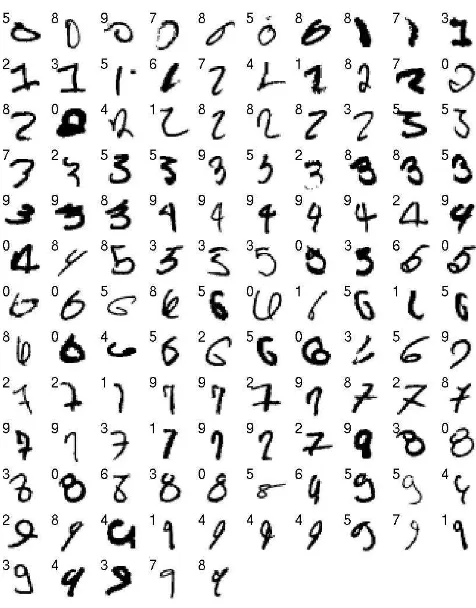
Figure 7: The 125 test cases that the network got wrong. Each case is labeled by the network’s guess. The true classes are arranged in standard scan order.
In the initial phase of training, the greedy algorithm de-scribed in section 4 was used to train each layer of weights separately, starting at the bottom. Each layer was trained for 30 sweeps through the training set (called “epochs”). Dur-ing trainDur-ing, the units in the “visible” layer of each RBM had real-valued activities between 0 and 1. These were the nor-malized pixel intensities when learning the bottom layer of weights. For training higher layers of weights, the real-valued activities of the visible units in the RBM were the activation probabilities of the hidden units in the lower-level RBM. The hidden layer of each RBM used stochastic binary values when that RBM was being trained. The greedy training took a few hours per layer in Matlab on a 3GHz Xeon processor and when it was done, the error-rate on the test set was 2.49% (see below for details of how the network is tested).
picking unitiwas given by:
where xi is the total input received by unit i. Curiously,
the learning rules are unaffected by the competition between units in a softmax group, so the synapses do not need to know which unit is competing with which other unit. The competi-tion affects the probability of a unit turning on, but it is only this probability that affects the learning.
After the greedy layer-by-layer training, the network was trained, with a different learning rate and weight-decay, for 300 epochs using the up-down algorithm described in section 5. The learning rate, momentum, and weight-decay7 were chosen by training the network several times and observing its performance on a separate validation set of 10,000 im-ages that were taken from the remainder of the full training set. For the first 100 epochs of the up-down algorithm, the up-pass was followed by three full iterations of alternating Gibbs sampling in the associative memory before perform-ing the down-pass. For the second 100 epochs, six iterations were performed, and for the last 100 epochs, ten iterations were performed. Each time the number of iterations of Gibbs sampling was raised, the error on the validation set decreased noticeably.
The network that performed best on the validation set was then tested and had an error rate of 1.39%. This network was then trained on all 60,000 training images8until its error-rate on the full training set was as low as its final error-rate had been on the initial training set of 44,000 images. This took a further 59 epochs making the total learning time about a week. The final network had an error-rate of 1.25%9. The
errors made by the network are shown in figure 7. The 49 cases that the network gets correct but for which the second best probability is within 0.3 of the best probability are shown in figure 6.
The error-rate of 1.25% compares very favorably with the error-rates achieved by feed-forward neural networks that have one or two hidden layers and are trained to optimize discrimination using the back-propagation algorithm (see ta-ble 1, appearing after the references). When the detailed connectivity of these networks is not hand-crafted for this
7
No attempt was made to use different learning rates or weight-decays for different layers and the learning rate and momentum were always set quite conservatively to avoid oscillations. It is highly likely that the learning speed could be considerably improved by a more careful choice of learning parameters, though it is possible that this would lead to worse solutions.
8
The training set has unequal numbers of each class, so images were assigned randomly to each of the 600 mini-batches.
9
To check that further learning would not have significantly im-proved the error-rate, the network was then left running with a very small learning rate and with the test error being displayed after ev-ery epoch. After six weeks the test error was fluctuating between 1.12% and 1.31% and was 1.18% for the epoch on which number of
trainingerrors was smallest.
particular task, the best reported error-rate for stochastic on-line learning with a separate squared error on each of the 10 output units is 2.95%. These error-rates can be reduced to 1.53% in a net with one hidden layer of 800 units by using small initial weights, a separate cross-entropy error function on each output unit, and very gentle learning (John Platt, per-sonal communication). An almost identical result of 1.51% was achieved in a net that had 500 units in the first hidden layer and 300 in the second hidden layer by using “soft-max” output units and a regularizer that penalizes the squared weights by an amount that is carefully chosen using a valida-tion set. For comparison, nearest neighbor has a reported er-ror rate (http://oldmill.uchicago.edu/ wilder/Mnist/) of 3.1% if all 60,000 training cases are used (which is extremely slow) and 4.4% if 20,000 are used. This can be reduced to 2.8% and 4.0% by using an L3 norm.
The only standard machine learning technique that comes close to the 1.25% error rate of our generative model on the basic task is a support vector machine which gives an er-ror rate of 1.4% (Decoste and Schoelkopf, 2002). But it is hard to see how support vector machines can make use of the domain-specific tricks, like weight-sharing and sub-sampling, which LeCun et al. (1998) use to improve the per-formance of discriminative neural networks from 1.5% to 0.95%. There is no obvious reason why weight-sharing and sub-sampling cannot be used to reduce the error-rate of the generative model and we are currently investigating this ap-proach. Further improvements can always be achieved by av-eraging the opinions of multiple networks, but this technique is available to all methods.
Substantial reductions in the error-rate can be achieved by supplementing the data set with slightly transformed versions of the training data. Using one and two pixel translations Decoste and Schoelkopf (2002) achieve 0.56%. Using lo-cal elastic deformations in a convolutional neural network, Simard et al. (2003) achieve 0.4% which is slightly better than the0.63%achieved by the best hand-coded recognition algorithm (Belongie et al., 2002). We have not yet explored the use of distorted data for learning generative models be-cause many types of distortion need to be investigated and the fine-tuning algorithm is currently too slow.
6.2
Testing the network
One way to test the network is to use a stochastic up-pass from the image to fix the binary states of the 500 units in the lower layer of the associative memory. With these states fixed, the label units are given initial real-valued activities of 0.1and a few iterations of alternating Gibbs sampling are then used to activate the correct label unit. This method of testing gives error rates that are almost 1% higher than the rates re-ported above.
Figure 8: Each row shows 10 samples from the generative model with a particular label clamped on. The top-level asso-ciative memory is run for 1000 iterations of alternating Gibbs sampling between samples.
Almost all the computation required is independent of which label unit is turned on (Teh and Hinton, 2001) and this method computes the exact conditional equilibrium distribution over labels instead of approximating it by Gibbs sampling which is what the previous method is doing. This method gives er-ror rates that are about 0.5% higher than the ones quoted be-cause of the stochastic decisions made in the up-pass. We can remove this noise in two ways. The simplest is to make the up-pass deterministic by using probabilities of activation in place of stochastic binary states. The second is to repeat the stochastic up-pass twenty times and average either the la-bel probabilities or the lala-bel log probabilities over the twenty repetitions before picking the best one. The two types of av-erage give almost identical results and these results are also very similar to using a deterministic up-pass, which was the method used for the reported results.
7
Looking into the mind of a neural network
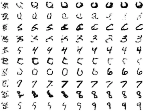
To generate samples from the model, we perform alternating Gibbs sampling in the top-level associative memory until the Markov chain converges to the equilibrium distribution. Then we use a sample from this distribution as input to the layers below and generate an image by a single down-pass through the generative connections. If we clamp the label units to a particular class during the Gibbs sampling we can see im-ages from the model’s class-conditional distributions. Figure 8 shows a sequence of images for each class that were gener-ated by allowing 1000 iterations of Gibbs sampling between samples.
We can also initialize the state of the top two layers by providing a random binary image as input. Figure 9 shows how the class-conditional state of the associative memory then evolves when it is allowed to run freely, but with the
Figure 9: Each row shows 10 samples from the generative model with a particular label clamped on. The top-level as-sociative memory is initialized by an up-pass from a random binary image in which each pixel is on with a probability of 0.5. The first column shows the results of a down-pass from this initial high-level state. Subsequent columns are produced by 20 iterations of alternating Gibbs sampling in the associa-tive memory.
label clamped. This internal state is “observed” by perform-ing a down-pass every 20 iterations to see what the associa-tive memory has in mind. This use of the word “mind” is not intended to be metaphorical. We believe that a mental state is the state of a hypothetical, external world in which a high-level internal representation would constitute veridical perception. That hypothetical world is what the figure shows.
8
Conclusion
We have shown that it is possible to learn a deep, densely-connected, belief network one layer at a time. The obvious way to do this is to assume that the higher layers do not ex-ist when learning the lower layers, but this is not compatible with the use of simple factorial approximations to replace the intractable posterior distribution. For these approximations to work well, we need the true posterior to be as close to facto-rial as possible. So instead of ignoring the higher layers, we assume that they exist but have tied weights which are con-strained to implement a complementary prior that makes the true posterior exactly factorial. This is equivalent to having an undirected model which can be learned efficiently using contrastive divergence. It can also be viewed asconstrained variational learning because a penalty term – the divergence between the approximate and true posteriors – has been re-placed by the constraint that the prior must make the varia-tional approximation exact.
com-plementary, so the true posterior distributions in lower layers are no longer factorial and the use of the transpose of the gen-erative weights for inference is no longer correct. Neverthe-less, we can use a variational bound to show that adapting the higher-level weights improves the overall generative model.
To demonstrate the power of our fast, greedy learning algorithm, we used it to initialize the weights for a much slower fine-tuning algorithm that learns an excellent gener-ative model of digit images and their labels. It is not clear that this is the best way to use the fast, greedy algorithm. It might be better to omit the fine-tuning and use the speed of the greedy algorithm to learn an ensemble of larger, deeper networks or a much larger training set. The network in figure 1 has about as many parameters as 0.002 cubic millimeters of mouse cortex (Horace Barlow,pers. comm.), and several hundred networks of this complexity could fit within a sin-gle voxel of a high resolution fMRI scan. This suggests that much bigger networks may be required to compete with hu-man shape recognition abilities.
Our current generative model is limited in many ways (Lee and Mumford, 2003). It is designed for images in which non-binary values can be treated as probabilities (which is not the case for natural images); its use of top-down feedback during perception is limited to the associative memory in the top two layers; it does not have a systematic way of dealing with per-ceptual invariances; it assumes that segmentation has already been performed and it does not learn to sequentially attend to the most informative parts of objects when discrimination is difficult. It does, however, illustrate some of the major ad-vantages of generative models as compared to discriminative ones:
1. Generative models can learn low-level features with-out requiring feedback from the label and they can learn many more parameters than discriminative mod-els without overfitting. In discriminative learning, each training case only constrains the parameters by as many bits of information as are required to specify the label. For a generative model, each training case constrains the parameters by the number of bits required to spec-ify the input.
2. It is easy to see what the network has learned by gener-ating from its model.
3. It is possible to interpret the non-linear, distributed rep-resentations in the deep hidden layers by generating im-ages from them.
4. The superior classification performance of discrimina-tive learning methods only holds for domains in which it is not possible to learn a good generative model. This set of domains is being eroded by Moore’s law.
Acknowledgments
We thank Peter Dayan, Zoubin Ghahramani, Yann Le Cun, Andriy Mnih, Radford Neal, Terry Sejnowski and Max Welling for helpful discussions and the referees for greatly improving the manuscript. The research was supported by
NSERC, the Gatsby Charitable Foundation, CFI and OIT. GEH is a fellow of the Canadian Institute for Advanced Re-search and holds a Canada ReRe-search Chair in machine learn-ing.
References
Belongie, S., Malik, J., and Puzicha, J. (2002). Shape match-ing and object recognition usmatch-ing shape contexts. IEEE Transactions on Pattern Analysis and Machine Intelli-gence, 24(4):509–522.
Carreira-Perpinan, M. A. and Hinton, G. E. (2005). On con-trastive divergence learning. InArtificial Intelligence and Statistics, 2005.
Decoste, D. and Schoelkopf, B. (2002). Training invariant support vector machines.Machine Learning, 46:161–190. Freund, Y. (1995). Boosting a weak learning algorithm by majority. Information and Computation, 12(2):256 – 285. Friedman, J. and Stuetzle, W. (1981). Projection pursuit re-gression. Journal of the American Statistical Association, 76:817–823.
Hinton, G. E. (2002). Training products of experts by minimizing contrastive divergence. Neural Computation, 14(8):1711–1800.
Hinton, G. E., Dayan, P., Frey, B. J., and Neal, R. (1995). The wake-sleep algorithm for self-organizing neural networks. Science, 268:1158–1161.
LeCun, Y., Bottou, L., and Haffner, P. (1998). Gradient-based learning applied to document recognition. Proceedings of the IEEE, 86(11):2278–2324.
Lee, T. S. and Mumford, D. (2003). Hierarchical bayesian in-ference in the visual cortex.Journal of the Optical Society of America, A., 20:1434–1448.
Marks, T. K. and Movellan, J. R. (2001). Diffusion networks, product of experts, and factor analysis. InProc. Int. Conf. on Independent Component Analysis, pages 481–485. Mayraz, G. and Hinton, G. E. (2001). Recognizing
hand-written digits using hierarchical products of experts.IEEE Transactions on Pattern Analysis and Machine Intelli-gence, 24:189–197.
Neal, R. (1992). Connectionist learning of belief networks. Artificial Intelligence, 56:71–113.
Neal, R. M. and Hinton, G. E. (1998). A new view of the EM algorithm that justifies incremental, sparse and other variants. In Jordan, M. I., editor,Learning in Graphical Models, pages 355—368. Kluwer Academic Publishers. Ning, F., Delhomme, D., LeCun, Y., Piano, F., Bottou, L.,
and Barbano, P. (2005). Toward automatic phenotyping of developing embryos from videos. IEEE Transactions on Image Processing, 14(9):1360–1371.
Roth, S. and Black, M. J. (2005). Fields of experts: A frame-work for learning image priors. InIEEE Conf. on Com-puter Vision and Pattern Recognition.
Sanger, T. D. (1989). Optimal unsupervised learning in a single-layer linear feedforward neural. Neural Networks, 2(6):459–473.
Simard, P. Y., Steinkraus, D., and Platt, J. (2003). Best prac-tice for convolutional neural networks applied to visual document analysis. InInternational Conference on Docu-ment Analysis and Recogntion (ICDAR), IEEE Computer Society, Los Alamitos, pages 958–962.
Teh, Y. and Hinton, G. E. (2001). Rate-coded restricted Boltz-mann machines for face recognition. InAdvances in Neu-ral Information Processing Systems, volume 13.
Teh, Y., Welling, M., Osindero, S., and Hinton, G. E. (2003). Energy-based models for sparse overcomplete representa-tions. Journal of Machine Learning Research, 4:1235– 1260.
Welling, M., Hinton, G., and Osindero, S. (2003). Learn-ing sparse topographic representations with products of Student-t distributions. In S. Becker, S. T. and Ober-mayer, K., editors,Advances in Neural Information Pro-cessing Systems 15, pages 1359–1366. MIT Press, Cam-bridge, MA.
9
Tables
Version of MNIST task Learning algorithm Test error % permutation-invariant Our generative model 1.25
784−>500−>500<−−>2000<−−>10
permutation-invariant Support Vector Machine 1.4 degree 9 polynomial kernel
permutation-invariant Backprop784−>500−>300−>10 1.51 cross-entropy & weight-decay
permutation-invariant Backprop784−>800−>10 1.53 cross-entropy & early stopping
permutation-invariant Backprop784−>500−>150−>10 2.95 squared error & on-line updates
permutation-invariant Nearest Neighbor 2.8 All 60,000 examples & L3 norm
permutation-invariant Nearest Neighbor 3.1 All 60,000 examples & L2 norm
permutation-invariant Nearest Neighbor 4.0 20,000 examples & L3 norm
permutation-invariant Nearest Neighbor 4.4 20,000 examples & L2 norm
unpermuted images Backprop 0.4
extra data from cross-entropy & early-stopping elastic deformations convolutional neural net
unpermuted deskewed Virtual SVM 0.56
images, extra data degree 9 polynomial kernel from 2 pixel transl.
unpermuted images Shape-context features 0.63 hand-coded matching
unpermuted images Backprop in LeNet5 0.8 extra data from convolutional neural net
affine transformations
Unpermuted images Backprop in LeNet5 0.95 convolutional neural net
10
Appendix
A
Complementary Priors
General complementarity
Consider a joint distribution over observables,x, and hidden variables,y. For a given likelihood function,P(x|y), we define the corresponding family of complementary priors to be those distributions,P(y), for which the joint distribution,P(x,y) = P(x|y)P(y), leads to posteriors,P(y|x), that exactly factorise, i.e. leads to a posterior that can be expressed asP(y|x) =
Q
jP(yj|x).
Not all functional forms of likelihood admit a complementary prior. In this appendix we will show that the following family constitutes all likelihood functions admitting a complementary prior:
P(x|y) = 1 Ω(y)exp
X
j
Φj(x, yj) +β(x)
= exp
X
j
Φj(x, yj) +β(x)−log Ω(y)
(11)
whereΩis the normalisation term. For this assertion to hold we need to assume positivity of distributions: that bothP(y)>0 andP(x|y)>0for every value ofyandx. The corresponding family of complementary priors then assume the form:
P(y) = 1 Cexp
log Ω(y) + X
j
αj(yj)
(12)
whereCis a constant to ensure normalisation. This combination of functional forms leads to the following expression for the joint:
P(x,y) = 1 Cexp
X
j
Φj(x, yj) +β(x) +
X
j
αj(yj)
(13)
To prove our assertion, we need to show that every likelihood function of the form in Eq. 11 admits a complementary prior, and also that complementarity implies the functional form in Eq. 11. Firstly, it can be directly verified that Eq. 12 is a complementary prior for the likelihood functions of Eq. 11. To show the converse, let us assume thatP(y)is a complementary prior for some likelihood functionP(x|y). Notice that the factorial form of the posterior simply means that the joint distribution P(x,y) = P(y)P(x|y)satisfies the following set of conditional independencies: yj ⊥⊥yk|xfor everyj 6=k. This set of
conditional independencies is exactly those satisfied by an undirected graphical model with an edge between every hidden variable and observed variable and among all observed variables (Pearl, 1988). By the Hammersley-Clifford Theorem, and using our positivity assumption, the joint distribution must be of the form of Eq. 13, and the forms for the likelihood function Eq. 11 and prior Eq. 12 follow from this.
Complementarity for infinite stacks
We now consider a subset of models of the form in Eq. 13 for which the likelihood also factorises. This means that we now have two sets of conditional independencies:
P(x|y) = Y
i
P(xi|y) (14)
P(y|x) = Y
j
P(yj|x) (15)
This condition is useful for our construction of the infinite stack of directed graphical models.
characterises all joint distributions of interest,
while the likelihood functions take on the form,
P(x|y) = exp
Although it is not immediately obvious, the marginal distribution over the observables,x, in Eq. 16 can also be expressed as an infinite directed model in which the parameters defining the conditional distributions between layers are tied together.
An intuitive way of validating of this assertion is as follows. Consider one of the methods by which we might draw samples from the marginal distributionP(x)implied by Eq. 16. Starting from an arbitrary configuration ofy we would iteratively perform Gibbs sampling using, in alternation, the distributions given in Eq. 14 and 15. If we run this Markov chain for long enough then, since our positivity assumptions ensure that the chain mixes properly, we will eventually obtain unbiased samples from the joint distribution given in Eq. 16.
Now let us imagine that we unroll this sequence of Gibbs updates in space — such that we consider each parallel update of the variables to constitute states of a separate layer in a graph. This unrolled sequence of states has a purely directed structure (with conditional distributions taking the form of Eq. 14 and 15 in alternation). By equivalence to the Gibbs sampling scheme, after many layers in such an unrolled graph, adjacent pairs of layers will have a joint distribution as given in Eq. 16.
We can formalize this intuition for unrolling the graph as follows. The basic idea is to construct a joint distribution by unrolling a graph “upwards” (i.e. moving away from the data-layer to successively deeper hidden layers), so that we can put a well-defined distribution over an infinite stack of variables. Then we verify some simple marginal and conditional properties of this joint distribution, and show that our construction is the same as that obtained by unrolling the graph downwards from a very deep layer.
Letx=x(0),y=y(0),x(1),y(1),x(2),y(2), . . .be a sequence (stack) of variables the first two of which are identified as our original observed and hidden variables, while x(i)andy(i) are interpreted as a sequence of successively deeper layers. First, define the functions
over dummy variablesy′ ,x′
. Now define a joint distribution over our sequence of variables (assuming first-order Markovian dependency) as follows:
We verify by induction that the distribution has the following marginal distributions:
P(x(i)) =f
x(x(i)) i= 0,1,2, . . . (26)
P(y(i)) =f
Fori= 0this is given by definition of the distribution in Eq. 23 and by Eqs. 19 and 20. Fori >0, we have:
P(x(i)) = X
y(i−1)
P(x(i)|y(i−1))P(y(i−1)) = X
y(i−1)
f(x(i),y(i−1))
fy(y(i−1))
fy(y(i
−1)) =f
x(x(i)) (28)
and similarly forP(y(i)). Now we see that the following “downward” conditional distributions also hold true:
P(x(i)|y(i)) =P(x(i),y(i))/P(y(i)) =gx(x(i)|y(i)) (29)
P(y(i)|x(i+1)) =P(y(i),x(i+1))/P(x(i+1)) =gy(y(i)|x(i+1)) (30)
So our joint distribution over the stack of variables also gives the unrolled graph in the “downward” direction, since the con-ditional distributions in Eq. 29 and 30 are the same as those used to generate a sample in a downwards pass and the Markov chain mixes.
Inference in this infinite stack of directed graphs is equivalent to inference in the joint distribution over the sequence of variables. In other words, givenx(0) we can simply use the definition of the joint distribution Eqs. 23, 24 and 25 to obtain a sample from the posterior simply by samplingy(0)|x(0),x(1)|y(0),y(1)|x(1),. . .. This directly shows that our inference procedure is exact for the unrolled graph.
B
Pseudo-Code For Up-Down Algorithm
We now present “MATLAB-style” pseudo-code for an implementation of the up-down algorithm described in section 5 and used for back-fitting. (This method is a contrastive version of the wake-sleep algorithm (Hinton et al., 1995).)
The code outlined below assumes a network of the type shown in Figure 1 with visible inputs, label nodes, and three layers of hidden units. Before applying the up-down algorithm, we would first perform layer-wise greedy training as described in sections 3 and 4.
\% UP-DOWN ALGORITHM \%
\% the data and all biases are row vectors.
\% the generative model is: lab <--> top <--> pen --> hid --> vis \% the number of units in layer foo is numfoo
\% weight matrices have names fromlayer_tolayer
\% "rec" is for recognition biases and "gen" is for generative biases. \% for simplicity, the same learning rate, r, is used everywhere.
\% PERFORM A BOTTOM-UP PASS TO GET WAKE/POSITIVE PHASE PROBABILITIES \% AND SAMPLE STATES
wakehidprobs = logistic(data*vishid + hidrecbiases); wakehidstates = wakehidprobs > rand(1, numhid);
wakepenprobs = logistic(wakehidstates*hidpen + penrecbiases); wakepenstates = wakepenprobs > rand(1, numpen);
postopprobs = logistic(wakepenstates*pentop + targets*labtop + topbiases); postopstates = waketopprobs > rand(1, numtop));
\% POSITIVE PHASE STATISTICS FOR CONTRASTIVE DIVERGENCE poslabtopstatistics = targets’ * waketopstates;
pospentopstatistics = wakepenstates’ * waketopstates;
\% PERFORM numCDiters GIBBS SAMPLING ITERATIONS USING THE TOP LEVEL \% UNDIRECTED ASSOCIATIVE MEMORY
negtopstates = waketopstates; \% to initialize loop for iter=1:numCDiters
negpenprobs = logistic(negtopstates*pentop’ + pengenbiases); negpenstates = negpenprobs > rand(1, numpen);
neglabprobs = softmax(negtopstates*labtop’ + labgenbiases);
end;
\% NEGATIVE PHASE STATISTICS FOR CONTRASTIVE DIVERGENCE negpentopstatistics = negpenstates’*negtopstates; neglabtopstatistics = neglabprobs’*negtopstates;
\% STARTING FROM THE END OF THE GIBBS SAMPLING RUN, PERFORM A
\% TOP-DOWN GENERATIVE PASS TO GET SLEEP/NEGATIVE PHASE PROBABILITIES \% AND SAMPLE STATES
sleeppenstates = negpenstates;
sleephidprobs = logistic(sleeppenstates*penhid + hidgenbiases); sleephidstates = sleephidprobs > rand(1, numhid);
sleepvisprobs = logistic(sleephidstates*hidvis + visgenbiases);
\% PREDICTIONS
psleeppenstates = logistic(sleephidstates*hidpen + penrecbiases); psleephidstates = logistic(sleepvisprobs*vishid + hidrecbiases); pvisprobs = logistic(wakehidstates*hidvis + visgenbiases); phidprobs = logistic(wakepenstates*penhid + hidgenbiases);
\% UPDATES TO GENERATIVE PARAMETERS
-hidvis = hidvis + r*poshidstates’*(data-pvisprobs); visgenbiases = visgenbiases + r*(data - pvisprobs);
penhid = penhid + r*wakepenstates’*(wakehidstates-phidprobs); hidgenbiases = hidgenbiases + r*(wakehidstates - phidprobs);
\% UPDATES TO TOP LEVEL ASSOCIATIVE MEMORY PARAMETERS
labtop = labtop + r*(poslabtopstatistics-neglabtopstatistics); labgenbiases = labgenbiases + r*(targets - neglabprobs);
pentop = pentop + r*(pospentopstatistics - negpentopstatistics); pengenbiases = pengenbiases + r*(wakepenstates - negpenstates); topbiases = topbiases + r*(waketopsates - negtopstates);
\%UPDATES TO RECOGNITION/INFERENCE APPROXIMATION PARAMETERS
hidpen = hidpen + r*(sleephidstates’*(sleeppenstates-psleeppenstates)); penrecbiases = penrecbiases + r*(sleeppenstates-psleeppenstates);