THE IMPACT OF FOREIGN DIRECT INVESTMENT ON ECONOMIC GROWTH IN INDONESIA, 1980-2004: A CAUSALITY APPROACH | Wahyudi | Journal of Indonesian Economy and Business 6309 68684 1 PB

(1)

Volume 24, Number 3, 2009, 311 – 327

THE IMPACT OF FOREIGN DIRECT INVESTMENT ON

ECONOMIC GROWTH IN INDONESIA, 1980-2004:

A CAUSALITY APPROACH

1

Setyo Tri Wahyudi

Faculty of Economics, Brawijaya University (setyo_triwahyudi@yahoo.com)

Abstract

Foreign investment, in addition to domestic investment, is one of the driving sources of a nation's economy, because of its ability to create jobs and allow the transfer of technology that in turn encourages economic growth. Significant role contributed by these investments, in the context of Indonesia, can be seen from its contribution to the national economy.

This study aims to determine the relationship between investment and economic growth in Indonesia. Using the data of Foreign Direct Investment (FDI) and GDP on 1980-2004 periods, and method of causality, this study tried to answer the question of whether investment causes economic growth or whether economic growth causes investment.

To examine the relationship between two variables, there are three steps test conducted, unit roots test (using the ADF test); co integration test (using the Johansen co integration test); and causality test (using the Granger Causality test). Conclusion indicated that investment affects economic growth.

Keywords: Foreign direct investment, economic growth, granger causality.

INTRODUCTION1

During the past two decades, foreign direct investment (hereafter FDI) has become increasingly important in the developing world, with a growing number of developing countries succeeding in attracting substantial and rising amounts of inward FDI. Braunstein and Epstein (2002) said that Investment has become an essential commodity to the economy of a country. It because the invest-ment can drive the economic sectors, thereby creating employment and enable technology transfer, and will encourage sustainable economic growth.

1_{This paper was presented in the}_{2nd IRSA International} Institute, Bogor, 22-23 July 2009.

(2)

Journal of Indonesian Economy and Business September 312

35

30

25

20

15

10

5

0

1993 1994 1995 1996 1997 1998 1999 2000 2001 2002 2003 2004 2005 2006 2007

Source: Bank of Indonesia (2007).

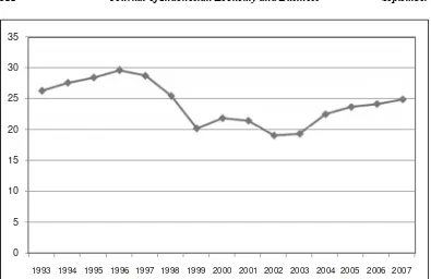
Figure 1. Contribution of Investment to GDP Growth

Source: Bank of Indonesia (2007).

Figure 2. Indonesia Investment Growth -40

-30 -20 -10 0 10 20 30

(3)

Less pulling of the investment growth and the occurrence of a decrease in the GDP contribution of the economic recovery of the crisis relatively more slowly than countries in the same conditions, such as South Korea and Thailand. Slowing investment growth is still associated with a variety of internal cons-traints, which is focused on un-conducive climate to invest. Insecurity problems, legal uncertainty, a complex bureaucracy to the condition of the infrastructure that do not support, still continues to be a major problem for investors. With various constraints, the investment performance tends to move moderate, with growth after the crisis in the bottom 15 percent.

In the theory, the economic theory has identified a number of channels through which FDI inflows may be beneficial to the host economy. Yet, the empirical literature has lagged behind and has had more trouble identifying these advantages in practice. The Government of Indonesia started liberalizing its capital account regime in 1967, when it introduced the Foreign Investment Law No. 1/1967. The government later adopted a free-floating foreign exchange system in 1970 which was followed by further liberalization of the financial sector in 1980s. Indonesia has since been largely perceived as an attractive destination for foreign investment and this relatively long exposure to investment flows makes it an ideal candidate for empirical research on their efficacy in generating econo-mic growth. Surprisingly, and in spite of the Indonesian government’s long-term interest in generating foreign investment inflows, very little has been done to evaluate their impact in the last 25 years (Khaliq & Noy, 2007). Moreover, almost all existing studies of the FDI-growth have concentrated on the aggregate growth effects of FDI in spite of the theoretical and ambiguities that have been developed over the recent decades. To the best of our knowledge, only several papers have looked at the impact of FDI at the Indonesian

case (see e.g Fry, 1993; Hill, 1998; Asafu-Adjaye, 2000; and Khaliq & Noy, 2007).

The main objective of this paper is, therefore, to test for the direction of causality between foreign direct investment (FDI) and economic growth (GDP) in the case of Indo-nesia. Then the questions that are ultimately addressed: 1) Did FDI lead to economic growth?; 2) Did economic growth lead to FDI in Indonesia?; 3) Did there are two way causal link between FDI and economic growth in Indonesia (or possibly no causality at all)?. To reach the objectives, this paper used Granger causality test method developed by Feridun (2002) and Feridun & Sissoko (2006) to test the direction of causality between the two variables.

The paper is organized as follows. Section 2 summarized the causality between FDI and Economic Growth. Section 3 provides the empirical studies related FDI and Economic growth. Section 4 introduces the methodology that provides a description of the data, models, and estimation. Section 5 presents the empi-rical results. Session 6 provides further dis-cussion on the results presented in the paper and concludes.

CAUSALITY BETWEEN FDI AND ECONOMIC GROWTH

(4)

practices and organizational arrangements (De Mello, 1999).

The conventional economic growth theories are being augmented by discussing growth in the context of an open rather than a closed economy, and the emergence of externality-based growth models. Even with the inclusion of FDI in the model of economic growth, traditional growth theories confine the possible impact of FDI to the short-run level of income, when actually recent research has increasingly uncovered an endogenous long-run role of FDI in economic growth determination.24According to the neo-classical models, FDI can only affect growth in the short run because of diminishing returns of capital in the long run.

In contrast with the conventional neo-classical model, which postulates that long run growth can only happen from the both exoge-nous labor force growth and technological progress, the rise of endogenous growth models (Barrow & Sala-i-Martin, 1995) made it possible to model FDI as promoting economic growth even in the long run through the permanent knowledge transfer that accompanies FDI. As an externality, this knowledge transfer, with other externalities, will account for the non-diminishing returns that result in long run growth (De Mello, 1997). Hence, if growth determinants, including FDI, are made endogenous in the model, long run effects of FDI will follow. Therefore, a particular channel whereby tech-nology spills over from advanced to lagging countries is the flow of FDI (Bengoa & Sanchez-Robles, 2003).

Nevertheless, most studies generally indicate that the effect of FDI on growth depends on other factors such as the degree of complementarity and substitution between domestic investment and FDI, and other country-specific characteristics. For instance,

2

For an excellent survey of such research, see De Mello (1997).

Buckley et al. (2002) argued that the extent to which FDI contributes to growth depends on the economic and social conditions in the recipient country. Countries with high rate of savings, open trade regime and high technolo-gical levels would benefit from increase FDI to their economies. Balasubramanyam et al. (1996) argued that FDI plays different role in the growth process due to the differing trade policy regimes.

However, FDI may have negative effect on the growth prospects of the recipient economy if they result in a substantial reverse flows in the form of remittances of profits, and dividends and/or if the multinational corpo-rations (MNCs) obtain substantial or other concessions from the host country. Bengoa & Sanchez-Robles (2003) argued that in order to benefit from long-term capital flows, the host country requires adequate human capital, sufficient infrastructure, and economic stability and liberalized markets. The view that FDI fosters economic growth in the host country, provided that the host country is able to take advantage of its spillovers is supported by empirical findings in De Mello (1999) and Obwona (2001). Borensztein et al. (1998) go further to suggest that FDI is an important vehicle for the transfer of technology, contri-buting relatively more to growth than domestic investment. They use a model of endogenous growth, in which the rate of technological progress is the main determinant of the long-term growth rate of income. Borensztein et al. (1998) point out that the contribution of FDI to economic growth is enhanced by its interac-tion with the level of human capital in the host country.

(5)

EMPIRICAL STUDIES

In the literature on the link between FDI and economic growth, Fry (1993) investigated the effects of FDI on five ASEAN countries (Indonesia, Malaysia, Philippine, Thailand, and Singapore) using cross-section data. He found that FDI was positively related to domestic investment but negatively related to domestic savings. Fry concluded that FDI could stimulate imports more than exports, resulting in a negative trade balance. However, overall, it has a positive effect on GDP growth. Meanwhile, Blomstr¨om et al. (1994) stated that FDI was positive and significant only for higher income countries and that is has no impact in lower income countries.

Hill (1998) examined the relationship between FDI and industrialization in Indonesia for the period 1967 to 1985. Foreign firms in the sample were found to be relatively more productive than domestic firms in the terms of capital intensity and technology utilization. He found technology transfer to be one of the benefits of FDI in Indonesia. De Mello (1999) attempted to find support for an FDI-led growth hypothesis when time series analysis and panel data estimation for a sample of 32 OECD and non-OECD countries covering the period 1970-1990 were made. He estimates the impact of FDI on capital accumulation and output growth in the recipient economy.

Asafu-Adjaye (2000) estimated the effects of FDI on Indonesia’s economic growth for the period 1970 to 1996. The results suggest that FDI, net private capital, human capital, and gross domestic saving jointly influence economic growth. FDI has a significant positive effect on economic growth, while net private capital has no significant effect. Boon (2001) investigated the causal relationship between FDI and economic growth in Malaysia. He found that bidirectional causality exist, between FDI and economic growth in Malaysia, i.e while growth in GDP attracts FDI, FDI also contributes to an increase output.

Chakraborty and Basu (2002) investigated the two-way link between foreign direct investment and growth for India using a structural cointegration model with vector error correction mechanism. The resulting cointegrating vectors indicate that the VECM model reveals three important features: (a) GDP in India is not Granger caused by FDI; the causality runs more from GDP to FDI; (b) trade liberalization policy of the Indian government had some positive short run impact on the FDI; and (c) FDI tends to lower the unit labor cost suggesting that FDI in India is labor displacing.

Feridun (2002) examines the relationships between foreign direct investment and GDP per capita in the economy of Cyprus, using the methodology of Granger causality and vector auto regression (VAR). Strong evidence emer-ges that the economic growth as measured by GDP in Cyprus is Granger caused by the FDI, but not vice versa. Results further suggest that Cyprus’s capacity to progress on economic development will depend on the country’s performance in attracting foreign capital. Feridun and Sissoko (2006) examined the relationship between foreign direct investment and GDP per capita in the economy of Singapore, using the methodology of Granger causality and vector auto regression (VAR). Strong evidence emerges that the economic growth as measured by GDP in Singapore is Granger caused by the FDI. Results further suggest that Singapore’s capacity to progress on economic development will depend on the country’s performance in attracting foreign capital.

(6)

growth indeed attracts FDI influx, which supports the market-size hypothesis; while the FDI influx stimulates the economic growth of China to some degree, the result is not significant.

Khaliq and Noy (2007) investigates the impact of foreign direct investment (FDI) on economic growth using detailed sectoral data for FDI inflows to Indonesia over the period 1997-2006. The sectors examined were: farm food crops, livestock product, forestry, fishery, mining and quarrying, non-oil and gas indus-try, electricity, gas and water, construction, retail and wholesale trade, hotels and restaurant, transport and communications, and other private and services sectors. In the aggregate level, FDI was observed to have a positive effect on economic growth. However, when accounting for the different average growth performance across sectors, the beneficial impact of FDI is no longer apparent. When examining different impacts across sectors, estimation results show that the composition of FDI matters for its effect on economic growth with very few sectors is showing positive impact of FDI and one sector even showing a robust negative impact of FDI inflows (mining and quarrying).

At least, based on the theoretical review and empirical study that has been done, there are two important summary points associated with this study that are 1) the debate about whether the FDI impact on EG or vice versa, perhaps, due to the different use of proxy variables. Differences in used of proxy absolutely will give different results too, for example FDI can be represented by FDI inflows and FDI outflows, as well as for EG can be represented by GDP per capita, real GDP, and GDP growth; and 2) as described by Buckley et al, (2002) stated that the contri-bution of both is also influenced by social and other economic factors in each country as the research sample. That means, besides the use of different proxy of variables, the characteristics of state/country also will give

affect the relationship between those variables. Therefore, in this study, once again trying to emphasize on how the relationship between two variables above for the sample of developing countries, especially Indonesia, and uses real data of FDI and real GDP growth, respectively as the proxy and proxy EG FDI.

METHODOLOGY

1. Definition

In analyzing the contribution of FDI to EG, it is necessary to know the type of investment that qualifies as FDI and to know the definition of the EG.

a. Foreign Direct Investment (FDI)

Foreign direct investment does not include all investments across border. There are some features that make foreign direct investment different from other international investments. FDI is the investment made by a company outside its home country. It is the flow of long-term capital based on long term profit consideration involved in international produc-tion (Caves, 1996). Lipsey (1999) said interna-tionalized production arises from foreign direct investment. According to him, this is the investment that involves some degree of control of the acquired or created firm which is in any other country apart from the inves-tors’ country. This involvement in the control of the investment is the main feature that distinguishes FDI from portfolio investment. In this study, we use real FDI during 1980 to 2004 data for Indonesia.

b. Economic Growth (EG)

(7)

base year are used to reflect domestic econo-mic growth of the country for every year.

2. The Data

The real GDP data are obtained from the International Financial Statistic (IFS) yearly books and real foreign direct investment net inflows data was taken from the Global Market Information Database (GMID) web-site. Annual time series data covering the period 1980-2004 for which data was available was used.

3. Econometric Techniques

In order to examine the question men-tioned before, suitable econometric models are required. Since the objective of this research is to test the causality of variables, the test should be based on the appropriate multi-variate times series models. In doing so, the author employ the most frequently used Augmented Dickey-Fuller (ADF) unit root test to test for the non-stationarity of the series on the levels and the first difference. Then, if order of integration of the variables has been determined, the Johansen (1988) techniques can be applied to investigate cointegration among the variables. If the Johansen cointe-gration test shows no evidence of cointegra-tion between such variables then we can proceed to apply the Granger Causality test to assess hypothesis of causality between growth and FDI in Indonesia.

Following Feridun (2002) and Feridun & Sissoko (2006), completes of the examination procedures conducted in this paper can be described as follows: the econometric metho-dology firstly examines the stationary properties of the univariate time series. The present study uses the Augmented Dickey-Fuller (ADF) unit root test to examine the stationarity of the data series. It consists of running a regression of the first difference of the series against the series lagged once, lagged difference terms and optionally, a

constant and a time trend. This can be expressed as:

The test for a unit root is conducted on the coefficient of yt-1 in the regression. If the

coefficient is significantly different from zero then the hypothesis that y contains a unit root is rejected. Rejection of the null hypothesis implies stationarity.

Secondly, time series have to be examined for cointegration. Cointegration analysis helps to identify long-run economic relationships between two or several variables and to avoid the risk of spurious regression. Cointegration analysis is important because if two non-stationary variables are cointegrated, a VAR model in the first difference is misspecified due to the effect of a common trend. If a cointegration relationship is identified, the model should include residuals from vectors (lagged one period) in the dynamic vector error correcting mechanism (VECM) system. In this stage, Johansen (1988) cointegration test is used to identify cointegrating relation-ships among the variables. Within the Johansen multivariate cointegrating frame-work, the following system is estimated:

T containing the r cointegrating relationships and α carrying the corresponding adjustment coefficients in each of the r vectors. The Johansen approach can be used to carry out Granger causality test as well. In the Johansen framework, the first step is the estimation of an unrestricted, closed p-th order VAR in k

(8)

statis-Journal of Indonesian Economy and Business September 318

tics to determine the cointegration rank. The first of these is known as the trace statistic:

Trace (r0/k) = -T

∑

depending upon stage in the sequence. This is the relevant test statistic for the null hypothesis r £ r0 against the alternative r3r0+1. The second test statistic is the maximum eigenvalues test known as λmax; we denote it as

λmax (r0). This is closely related to the trace statistic but arises from changing the alternative hypothesis from r r ≥ r0 + 1. The idea is to try and improve the power of the test by limiting the alternative to a cointegration rank which is just one more than under the null hypothesis. The λmaxtest statistic is:

λmax (r0) = -T in (1- λi) for i

= r0 + 1 (4)

The null hypothesis is there are r cointegrating vectors, against the alternative of

r+1 cointegrating vectors. Johansen and Juselius (1990) indicated that the trace test might lack the power relative to the maximum eigenvalue test. Based on the power of the test, the maximum eigenvalue test statistic is often preferred. According to Granger (1969), Y said to “Granger-cause” X if and only if is better predicted by using the past values of Y than by not doing so with the past values of X being used in either case. In short, if scalar Y can help to forecast another scalar X, then we say that Y Granger-causes X. If Y causes X and X

does not cause Y, it is said that unidirectional causality exists from Y to X. If Y does not cause X and X does not cause Y, then X and Y

are statistically independent. If Y cause X and

X causes Y, it is said that feedback exists between X and Y. Essentially, Granger’s definition of causality is framed in terms of predictability.

To implement Granger test, we assume a particular autoregressive lag length k (or p) and estimate Equation (5) and (6) by OLS:

t

F-test is carried out for the null hypothesis of no Granger causality H0: bi1 = bi2 = ... = bik =

0, i = 1, 2. H0: bi1 = bi2 = bik = 0, i = 1, 2

where, F-statistic is the Wald statistic for the null hypothesis. If the F-statistic is greater than a certain critical value for an F

distribution, then we reject the null hypothesis that Y does not Granger-cause X (equation (1)), which means Y Granger-causes X.

A time series with stable mean value and standard deviation is called a stationary series. If d differences have to be made to produce a stationary process, then it can be defined as integrated of order d. Engle and Granger (1987) state that if several variables are all I(d)

series, their linear combination may be cointegrated, that is, their linear combination may be stationary. Although the variables may drift away from equilibrium for a while, economic forces may be expected to act so as to restore equilibrium, thus, they tend to move together in the long run irrespective of short run dynamics. The definition of the Granger causality is based on the hypothesis that X and

(9)

direction of causality can be decided upon via standard F-tests in the first differenced VAR. The VAR in the first difference can be written as:

EMPIRICAL RESULT AND ANALYSIS

Since many economic variables are non-stationary time series, we need to pretest the variables for their order of integration before verifying the cause-and-effect relation of the time series. The empirical results are reported in three steps. First, we establish that both FDI and GDP have unit roots. In the second step, we look for cointegration using Johansen Cointegration test developed by Johansen (1988). Finally, we look the causality between FDI and GDP using Granger causality test developed by Granger (1969). The summa-rized of the results for each step as follows: Unit Root Test

The objective of the unit root test is to empirically examine whether a series contains a unit root. If the series contains a unit root, this means that the series is non-stationary. Otherwise, the series will be categorized as stationary. The common method to test the presence of a unit root is the Dickey-Fuller or Augmented Dickey-Fuller test (ADF test).

The unit root tests results contain a

constant and a linear time trend for the series in levels and first difference. Constant and

linear time trend was the right choice of conducting unit root testing because this method can best explain a certain time trend

that was found among the data during 25 years period. The ADF test with trend and without trend, for both level and first difference, as shown in column 1, 2, 3, and 4 are examined respectively as presented in Table 1.

The results of the unit root tests are reported in the Table 1. As is apparent from the table, by applying Augmented Dickey-Fuller (ADF) unit root tests3 in the level and differenced forms, the result of the stationary check as presented in the Table 1, indicates that all the series are non-stationary at the 1 percent and 5 percent level of significance. The rejection of the stationary at this level leads to testing of the first differences of variables. The test results for first differences show that all series are stationary at 1 percent and 5 percent significance.Based on these test results, it is, therefore we can conclude the strong evidence emerges that all the time series are I (1).

Johansen Cointegration Test

In the next step, we use Johansen Cointe-gration technique based on Johansen (1988) which uses a residual-based ADF test. This technique can be applied to investigate cointegration among the variables. Table 2 summarizes the output of the cointegration analyses as follow.

Cointegration necessitates that variables be integrated of the same order. Since all the data series were integrated processes of order one (I(1)), the linear combination (cointe-grating vectors) of one or more of these series may exhibit a long-run equilibrium relation-ships namely a cointegration relationship, among the variables. The cointegration test applies the test method of cointegration log likelihood ratio (LR) brought forward by Johansen (1988). The null hypothesis of the method is Ho : there are at most r cointegration relationships. The trace statistic amount of the test as presented in the Equation 3.

3_{For further result of Unit Root test results, read}

(10)

Table 1. Unit Root Test Results

H0: unit roots test I(1); H1: trend stationary I(0)

Level First Difference

Variable

Constant, No Trend

Constant & Trend

Constant, No Trend

Constant & Trend

Real GDP 0.9883 0.1348 0.0081** 0.0284**

Real FDI 0.0722 0.2310 0.0345** 0.1329

Note: The optimal lags for conducting the ADF tests were determined by AIC (Akaike information criteria). *(**) indicate significance at the 1% (5%) levels.

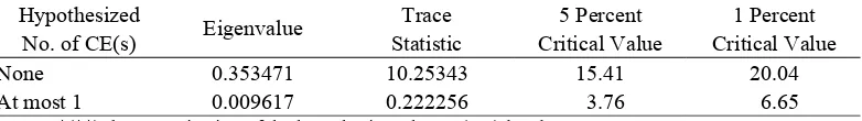
Table 2. Johansen Cointegration Test Results

Sample(adjusted): 1982 2004

Included observations: 23 after adjusting endpoints Trend assumption: Linear deterministic trend Series: RGDP RFDI

Lags interval (in first differences): 1 to 1 Unrestricted Cointegration Rank Test

Hypothesized Trace 5 Percent 1 Percent

No. of CE(s) Eigenvalue Statistic Critical Value Critical Value

None 0.353471 10.25343 15.41 20.04

At most 1 0.009617 0.222256 3.76 6.65

Notes: *(**) denotes rejection of the hypothesis at the 5%(1%) level Trace test indicates no cointegration at both 5% and 1% levels Source: Processed Data.

Based on the results in the Table 2, the Johansen cointegration trace test statistic, has strongly not rejected the null hypothesis of no cointegration (r=0), as well as the null of at most one cointegrating vector (r=1) at the 5 percent level of significance for the real GDP-real FDI relation. Neither trace nor eigenvalue statistic tests rejects the null hypothesis of no cointegration at the 5 percent level. Thus, given the results41, real GDP and real FDI appears not to have any long-run relationship, it only shows a short-run cointegration relationship.

Granger Causality Test

As FDI and GDP are cointegrated, we estimate Granger causality using the Engle and

4

For further result of Johansen Cointegration test results, read Appendix 2, on the latter part of this paper.

Granger (1987) method as alternative techni-ques of estimation to see the direction of causality as the last step. Results of the causality test are reported in the Table 3. The AIC criteria used to determine the appropriate lag length for the test equations, with a maximum of 4 lags considered. The samples for all Granger-causality tests begin in 1980 to 2004. Using a 5 percent level of significance, the results of Granger causality tests for this study presented as follow (Table 3).

As reported in the Table 3, the results of Granger-causality test52 show the null hypo-theses of real FDI does not granger cause real GDP is rejected in all of year lags, at the 5 percent and the 10 percent levels, respectively. On the other hand, the null hypotheses of real

5_{For further result of Granger Causality test results, read}

(11)

GDP does not granger cause real FDI is rejected in 1, 2 and 4 years lags, but not rejected in 3 year lags. This leads us to the conclusion that there is only a one-way causality running from real FDI to real GDP. Then we conclude that these results suggest that the direction of causality is from real FDI to real GDP since the estimated F value is significant at the 5 percent level; the critical F value is 3.39. On the other hand there is no reverse causation from real GDP to real FDI, since the computed F value is not statistically significant.

CONCLUSIONS

This paper has examined the relationship between real FDI and real GDP using time series data from the Indonesia economy. In Indonesia, FDI and growth has increased gradually since the 1980s. It is well known from the existing literature that FDI is major engine of growth in developing countries. Many of studies find a positive link between FDI and growth. But our econometric result shows that FDI inflows do not exert an independent influence on economic growth. And also the direction of causation is not towards from GDP growth to FDI but FDI to GDP growth. The use of proxy real FDI and real GDP growth in this study emphasized how the causal relationship between them that is FDI has a positive effect in influencing economic growth in Indonesia, especially during the period 1980-2004.

Base on these results, FDI has important to enhance economic growth in Indonesia

during the period of study. The importance of FDI cannot be overstated. As a result, the investment climate in the country must be improved through appropriate measures such as de-regulation in economic activity, increase domestic serving, developing the port net-work, road netnet-work, railways and telecommu-nication facilities etc, creating more trans-parency in the trade policy and more flexible labor markets and setting a suitable regulatory framework and tariff structure. Currently Indonesia provides an attractive investment regime but the response from the investor has not been very encouraging. If the ultimate objective of the government is to attract FDI for development, poverty reduction and growth, then an appropriate policy mix is necessary to achieve these.

REFERENCES

Asafu-Adjaye, John., 2000. “The effects of foreign direct investment on Indonesian economic growth, 1970-1996”. Economic Analysis and Policy, 30(1).

Balasubramanyam V.N., 1996. “Foreign direct investment in EP and IS countries”,

Economic Journal, 106, 92-105.

Barro, R. J. and X. Sala-i-Martin. 1995. “ Eco-nomic growth”. New York, McGraw-Hill. Bengoa, M. and Blanca Sanchez-Robles.

2003. “Foreign direct investment, econo-mic freedom and growth: New evidence from Latin America”. European Journal of Political Economy, 19, 529–545. Table 3. Granger Causality Test Results

F-Statistic

Null Hypothesis

Lag 1 Lag 2 Lag 3 Lag 4 RFDI does not Granger Cause RGDP 0.13222 0.57020 0.73433 0.81312 RGDP does not Granger Cause RFDI 0.08284 1.11112 3.3920** 3.2363

Notes: * Reject the null hypothesis at the 10% level. ** Reject the null hypothesis at the 5% level. Source: Processed Data.

(12)

Boon, Khor Chia., 2001. “Foreign direct investment and economics growth”.

Thesis. Graduate School of Economics. Universiti Utara Malaysia. Unpublished. Borensztein, E., de Gregorio, J., and J-W Lee,

1998. “How does foreign direct invest-ment affect economic growth?”. Journal of international Economics, 45, 115-135. Buckley, P. J., J. Clegg, and C. Wang. 2002.

“The impact of inward FDI on the performance of Chinese manufacturing firms”. Journal of International Business Studies, 33(4), 637–655.

Chakraborty, C., and Basu, P., 2002. “Foreign direct investment and growth in India: a cointegration approach”. Applied Econo-mics, 34, 1061-1073.

Caves R.E., 1996. “Multinational enterprise

and economic analysis”. New York:

Cambridge University press.

De Mello, L.R., Jr., 1997. “Foreign direct investment in Developing Countries: A selective survey”. Journal of Development Studies, 34(1), 1–34.

De Mello, L.R., Jr., 1999. “Foreign direct investment-led growth: Evidence from time series and panel data”. Oxford Economic Papers, 51(1), 133–151. Durham, B., 2004. “Absorptive capacity and

the effects of FDI and equity foreign portfolio investment on economic growth”. European Economic Review, 48, 285-306.

Engle, A. and Granger, C. (1987). “Cointegra-tion and error correc“Cointegra-tion: representa“Cointegra-tion, estimation and testing”. Econometrica, 55, 251-76.

Fry, M.J., 1993. “Foreign direct investment in Southeast Asia: Different impacts”. ISEAS

Current Economics Affairs series,

ASEAN Economic Research Unit, Institu-te of Southeast Asian Studies, Singapore. Feridun, M., 2002. “Foreign direct investment

and economic growth: A causality

analysis for Cyprus, 1976-2002”. Journal of Applied Sciences, 4(4), 654-657.

Feridun, M., Sissoko, Y., 2006. “Impact of FDI on economic development: a causality analysis for Singapore, 1976 – 2002”. MPRA Paper, 1054. Available at: http://mpra.ub.uni-muenchen.de/1054 Granger C., 1969. “Investigating casual

relationship by econometric models and cross spectral methods”. Econometrica, 37, 424-458.

Hassapis, C., Pittis, N. and Prodromidis, K., 1999. “Unit roots and granger causality in the EMS interest rates: the German dominance hypothesis revisited”. Journal of International Money and Finance, 18, 47-73.

Hill, H., 1988. “Foreign investment and indus-trialization in Indonesia”. Singapore: Oxford University press.

Johansen, S., 1988. “Statistical analysis of cointegrating vectors”. Journal of Eco-nomic Dynamics and Control, 12, 231-54. Johansen, S., Juselius, K., 1990. “Maximum

likelihood estimation and inference on cointegration with applications for the demand for money”. Oxford Bulletin of Economics and Statistics, 52, 169-210. Indonesian Investment Coordinating Board

(BKPM), 2006. “Fact and Figures”, avalaible at: www.bkpm.go.id

Jackson, J. and McIver, R., 2004. Macroeco-nomics, 7th eds. McGraw-Hill: Australia. Lipsey R.E., 1999. “The United States and

Europe as suppliers and recipients of FDI”. National Bureau of Economic Research, City University of New York (Pavia Conference).

Obwona, M., 2001. “Determinants of FDI and their impact on economic growth in Uganda”. African Development Review,

13, 46– 81.

(13)

APPENDIX

A. Unit Root Test

1. Real GDP

Augmented Dickey-Fuller test: Level (Constant, No Trend)

Null Hypothesis: RGDP has a unit root Exogenous: Constant

Lag Length: 0 (Automatic based on AIC, MAXLAG=1)

t-Statistic Prob.*

Augmented Dickey-Fuller test statistic 0.654525 0.9883 Test critical values: 1% level -3.737853

5% level -2.991878

10% level -2.635542

*MacKinnon (1996) one-sided p-values.

Augmented Dickey-Fuller test: Level (Constant & Trend)

Null Hypothesis: RGDP has a unit root Exogenous: Constant, Linear Trend

t-Statistic Prob.* Augmented Dickey-Fuller test statistic -3.073005 0.1348 Test critical values: 1% level -4.394309

5% level -3.612199

10% level -3.243079

Augmented Dickey-Fuller test: 1st Difference (Constant, No Trend)

Null Hypothesis: D(RGDP) has a unit root Exogenous: Constant

5% level -2.998064

10% level -2.638752

(14)

Augmented Dickey-Fuller test: 1st Difference (Constant & Trend)

Null Hypothesis: D(RGDP) has a unit root Exogenous: Constant, Linear Trend

5% level -3.622033

10% level -3.248592

*MacKinnon (1996) one-sided p-values. Source: Processed Data.

2. Real FDI

Augmented Dickey-Fuller test: Level (Constant, No Trend)

Null Hypothesis: RFDI has a unit root Exogenous: Constant

5% level -2.998064

10% level -2.638752

Augmented Dickey-Fuller test: Level (Constant & Trend)

Null Hypothesis: RFDI has a unit root Exogenous: Constant, Linear Trend

5% level -3.622033

10% level -3.248592

(15)

Augmented Dickey-Fuller test: 1st Difference (Constant, No Trend)

Null Hypothesis: D(RFDI) has a unit root Exogenous: Constant

5% level -2.998064

10% level -2.638752

Augmented Dickey-Fuller test: 1st Difference (Constant & Trend)

Null Hypothesis: D(RFDI) has a unit root Exogenous: Constant, Linear Trend

5% level -3.622033

10% level -3.248592

(16)

B. Johansen Cointegration Test

Sample(adjusted): 1982 2004

Included observations: 23 after adjusting endpoints Trend assumption: Linear deterministic trend Series: RGDP RFDI

Lags interval (in first differences): 1 to 1 Unrestricted Cointegration Rank Test

Hypothesized Trace 5 Percent 1 Percent

No. of CE(s) Eigenvalue Statistic Critical Value Critical Value None 0.353471 10.25343 15.41 20.04 At most 1 0.009617 0.222256 3.76 6.65

*(**) denotes rejection of the hypothesis at the 5%(1%) level Trace test indicates no cointegration at both 5% and 1% levels

Hypothesized Max-Eigen 5 Percent 1 Percent

No. of CE(s)

Eigenvalue

Statistic Critical Value Critical Value None 0.353471 10.03117 14.07 18.63 At most 1 0.009617 0.222256 3.76 6.65

*(**) denotes rejection of the hypothesis at the 5%(1%) level

Max-eigenvalue test indicates no cointegration at both 5% and 1% levels

Unrestricted Cointegrating Coefficients (normalized by b'*S11*b=I): RGDP RFDI

3.08E-06 1.85E-07 9.53E-06 -4.58E-08

Unrestricted Adjustment Coefficients (alpha):

D(RGDP) -4901.561 2225.220

D(RFDI) -2316273. 59482.37

1 Cointegrating Equation(s): Log likelihood -638.6355 Normalized cointegrating coefficients (std.err. in parentheses)

RGDP RFDI 1.000000 0.060146

(0.01918)

Adjustment coefficients (std.err. in parentheses) D(RGDP) -0.015102

(0.01671)

D(RFDI) -7.136396

(17)

C. Granger Causality Test

Pairwise Granger Causality Tests Lags: 1

Null Hypothesis: Obs F-Statistic Probability RFDI does not Granger Cause RGDP 24 0.13222 0.71977 RGDP does not Granger Cause RFDI 0.08284 0.77631

Pairwise Granger Causality Tests Lags: 2

Null Hypothesis: Obs F-Statistic Probability RFDI does not Granger Cause RGDP 23 0.57020 0.57530 RGDP does not Granger Cause RFDI 1.11112 0.35074 Pairwise Granger Causality Tests

Lags: 3

Null Hypothesis: Obs F-Statistic Probability RFDI does not Granger Cause RGDP 22 0.73433 0.54760 RGDP does not Granger Cause RFDI 3.39209 0.04583 Pairwise Granger Causality Tests

Lags: 4