HASL A new approach for performance eval

Contents lists available atScienceDirect

Performance Evaluation

journal homepage:www.elsevier.com/locate/peva

HASL: A new approach for performance evaluation and

model checking from concepts to experimentation

Paolo Ballarini

a

,

Benoît Barbot

b

,

Marie Duflot

c

,

Serge Haddad

b

,

Nihal Pekergin

d,∗

a_{Ecole Centrale de Paris, France} b_{LSV, ENS Cachan & CNRS & INRIA, France} c_{Université de Lorraine- LORIA, Nancy, France}

d_{LACL, Université Paris-Est Créteil, France}

a r t i c l e i n f o

Article history:

Received 23 May 2014

Received in revised form 31 January 2015 Accepted 20 April 2015

Available online xxxx

Keywords:

Discrete event stochastic process Statistical model checking Performance evaluation

a b s t r a c t

We introduce the Hybrid Automata Stochastic Language (HASL), a new temporal logic formalism for the verification of Discrete Event Stochastic Processes (DESP). HASL employs a Linear Hybrid Automaton (LHA) to select prefixes of relevant execution paths of a DESP. LHA allows rather elaborate information to be collectedon-the-flyduring path selection, providing the user with powerful means to express sophisticated measures. A formula of HASL consists of an LHA and an expressionZreferring to moments ofpath random variables. A simulation-based statistical engine is employed to obtain a confidence interval estimate of the expected value ofZ. In essence, HASL provides a unifying verification framework where temporal reasoning is naturally blended with elaborate reward-based analysis. Moreover, we have implemented a tool, named Cosmos, for performing analysis of HASL formula for DESP modelled by Petri nets. Using this tool we have developed two detailed case studies: a flexible manufacturing system and a genetic oscillator.

©2015 Elsevier B.V. All rights reserved.

1. Introduction

From model checking to quantitative model checking. Since its introduction [1], model checking has quickly become a prominent technique for verification of discrete-event systems. Its success is mainly due to three factors: (1) the ability to express specific properties by formulas of an appropriate logic, (2) the firm mathematical foundations based on automata theory and (3) the simplicity of the verification algorithms which has led to the development of numerous tools. While the study of systems requires both functional, performance and dependability analysis, originally the techniques associated with these kinds of analysis were different. However, in the mid nineties, classical temporal logics were adapted to express properties of Markov chains and verification procedures have been designed based on transient analysis of Markov chains [2].

From numerical model checking to statistical model checking. The numerical techniques for quantitative model checking are rather efficient when a memoryless property can be exhibited (or recovered by a finite-state memory), limiting the combinatory explosion due to the necessity to keep track of the history. Unfortunately both the formula associated with an

∗_{Corresponding author.}

E-mail address:nihal.pekergin@u-pec.fr(N. Pekergin).

http://dx.doi.org/10.1016/j.peva.2015.04.003

elaborated property and the stochastic process associated with a real application make rare the possibility of such a pattern. In these cases, statistical model checking [3] is an alternative to numerical techniques. Roughly speaking, statistical model checking consists in sampling executions of the system (possibly synchronised with some automaton corresponding to the formula to be checked) and comparing the ratio of successful executions with a threshold specified by the formula. The advantage of statistical model checking is the small memory requirement while its drawback is its inability to generate samples for execution paths of potentially unbounded length.

Limitations of existing logics. A topic that has not been investigated is the suitability of the temporal logic to express (non necessarily boolean) quantities defined by path operators (minimum, integration, etc.) applied on instantaneous indicators. Such quantities naturally occur in standard performance evaluation. For instance, the average length of a waiting queue during a busy period or the mean waiting time of a client are typical measures that cannot be expressed by the quantitative logics based on the concept of successful execution probability like CSL [4].

Our contribution. Following the idea to relieve these limitations, we introduce a new language called Hybrid Automaton Stochastic Language (HASL) which provides a unified framework both for model checking and for performance and dependability evaluation.1_{Evaluating a system using HASL allows both the probability computation of a complex set of paths}

as well as elaborate performability measures. The use of conditional expectation over these subsets of paths significantly enlarges the expressive power of the language.

A formula of HASL consists of an automaton and an expression. The automaton is a Linear Hybrid Automaton (LHA), i.e. an automaton with clocks, called in this contextdata variables, where the dynamic of each variable (i.e. the variable’s evolution) depends on the model states. This automaton is synchronised with the model of the system, precisely selecting accepting paths while maintaining detailed information on the path through data variables. The expression is based on moments of path random variables associated to path executions. These variables are obtained by operators like time integration on data variables.

HASL extends the expressiveness of automaton-based CSL as CSLTA[6] and its extension to multi-clocks [7] with state and action rewards and sophisticated update functions especially useful for performance and dependability evaluation. On the other hand it extends reward enriched versions of CSL, (CSRL [8]) with a more elaborate selection of path executions, and the possibility to consider multiple rewards. Therefore HASL makes possible to consider not only standard performability measures but also complex ones in a generic manner.

A statistical verification tool, named Cosmos, has been developed for this language. We have chosen generalised stochastic Petri nets (GSPN) as high level formalism for the description of the discrete event stochastic process since (1) it allows a flexible modelling w.r.t. the policies defining the process (choice, service and memory) and (2) due to the locality of net transitions and the simplicity of the firing rule it leads to efficient path generation. This tool has been presented in [9]. We have developed in this paper two detailed case studies relative to flexible manufacturing systems (FMS) and to gene expression. The choice of FMS was guided by the fact that they raise interesting analysis issues: productivity, flexibility, fault tolerance, etc. While analysis of such systems is usually based on standard performance indices, we demonstrate the usefulness of HASL through elaborate transient formulas. Similarly, biological measures often concern the shape of trajectories which can only be expressed by complex formulas. In addition, our experiments demonstrate the time efficiency of the Cosmostool.

Organisation. In Section2, we describe the class of stochastic models we refer to (i.e. DESP). In Section3, we formally introduce the HASL language and we provide an overview of the related work, where the expressiveness of HASL is compared with that of existing logics. Section4is dedicated to the presentation of the basic principles of statistical model checking as well as the Cosmos_{software tool for HASL verification. In Section5, we present two full case studies: a flexible manufacturing} system and a genetic oscillator. Finally, in Section6, we conclude and give some perspectives.

2. Discrete event stochastic process

We describe in this section a large class of stochastic models that are suitable for HASL verification, namely Discrete Event Stochastic Processes (DESP). Such a class includes in particular the main type of stochastic models targeted by existing stochastic logics, namely Markov chains. The definition of DESP we introduce is similar to that of generalised semi-Markov processes [10] as well as that given in [11].

Syntax. DESPs are stochastic processes consisting of a (possibly infinite) set of states and whose dynamic is triggered by a set of discrete events. We do not consider any restriction on the nature of the distribution associated with events. In the sequel dist

(

A

)

denotes the set of distributions whose support isA.

Definition 1. A DESP is a tuple

D

_{= ⟨}

_S

_{, π}

₀

_,

_E

_,

_Ind

_,

_enabled

_,

_delay

_,

_choice

_,

_target

_⟩

_where

•

Sis a (possibly infinite) set of states,

•

π

0

∈

dist

(

S

)

is the initial distribution on states,

•

Eis a finite set of events,

•

Indis a set of functions fromStoR_{called state indicators (including the constant functions),}

•

enabled

:

S

→

2E_{are the enabled events in each state with for alls}

_∈

_S,enabled

₍

_s

₎

_{̸= ∅}

_.

•

delay

:

S

×

E

→

dist

(

R+

₎

_{is a partial function defined for pairs}

₍

_s

_,

_e

₎

_{such thats}

_∈

_Sande

_∈

_enabled

₍

_s

₎

_.

•

choice

:

S

×

2E

_×

_R+

_→

_dist

₍

_E

₎

_{is a partial function defined for tuples}

₍

_s

_,

_E′

_,

_d

₎

_{such thatE}′

_⊆

_enabled

₍

_s

₎

_{and such that} the possible outcomes of the corresponding distribution are restricted toe

∈

E′.

•

target

:

S

×

E

×

R+

_→

_{Sis a partial function describing state changes through events defined for tuples}

₍

_s

_,

_e

_,

_d

₎

_such

thate

∈

enabled

(

s

)

.

From syntax to semantics. Given a states,enabled

(

s

)

is the set of events enabled ins. For an evente

∈

enabled

(

s

)

,delay

(

s

,

e

)

is the distribution of the delay between the enabling ofeand its possible occurrence. Furthermore, if we denotedthe earliest delay in some configuration of the process with states, andE′

_⊆

_enabled

₍

_s

₎

_{the set of events with minimal delay,} choice

(

s

,

E′

_,

_d

₎

_{describes how the conflict is randomly resolved: for alle}′

_∈

_E′

_,

_choice

₍

_s

_,

_E′

_,

_d

₎₍

_e′

₎

_{is the probability thate}′ will be selected amongE′_{after waiting for the delayd. The functiontarget}

₍

_s

_,

_e

_,

_d

₎

_{denotes the target state reached froms} on occurrence ofeafter waiting fordtime units.

Let us detail these explanations. Aconfigurationof a DESP is described as a triple

(

s

, τ ,

sched

)

withsbeing the current state,

τ

∈

R+_{the current time andsched}

_:

_E

_→

R+

_∪{+∞}

_{being the function that describes the occurrence time of each enabled}

event (

+∞

if the event is not enabled). Starting from a given configuration

(

s

, τ ,

sched

)

of a DESP, we can now informally define the dynamics of a DESP. It is an infinite loop, where each iteration consists in the following steps. First the function schedprovidesE′_{, the set of enabled events with minimal delay, i.e.E}′

_{= {}

_e

_∈

_enabled

₍

_s

₎

_{| ∀}

_e′

_∈

_enabled

₍

_s

_),

_sched

₍

_e

₎

_≤

sched

(

e′

)

}

. The corresponding delaydis equal tosched

(

s

)

−

τ

for anys

∈

E′. Then the probability distributionchoice

(

s

,

E′

,

d

)

randomly specifies which evente

∈

E′_{will be sampled. The next states}′_{is then defined bytarget}

₍

_s

_,

_e

_,

_d

₎

_{. Finally the function} schedis updated as follows. First for all eventse′_{different fromethat are still enabled,sched}

₍

_e′

₎

_{is maintained while for} all other enabled evente′_{in states}′_{, a new delayd}′_{is sampled according to the distributiondelay}

₍

_s′

_,

_e′

₎

_andsched

₍

_e′

₎

_is set to

τ

+

d

+

d′_{. Whene}′_{is disabled,sched}

₍

_e′

₎

_{is set to}

_+∞

_{. The three elements of a configuration being updated, the} system can now start a new iteration. Let us now give a more formal definition ofschedand the families of random variables corresponding to the successive states, events and time instants of a trace of the DESP.

Operational semantics of a DESP. Given a discrete event system, its execution is characterised by a (possibly infinite) sequence of events

{

e1

,

e2

, . . .

}

and occurrence time of these events. Only the events can change the state of the system. In the

stochastic framework, the behaviour of a DESP is defined by three families of random variables:

•

e1

, . . . ,

en

, . . .

defined over the set of eventsEdenoting the sequence of events occurring in the system;

•

s0

, . . . ,

sn

, . . .

defined over the (discrete) state space of the system, denoted asS.s0is the system initial state andsnfor

n

>

0 is the state reached after thenth event. The occurrence of an event does not necessarily modify the state of the system, and thereforesn+1may be equal tosn;

•

τ

0

≤

τ

1

≤ · · · ≤

τ

n

≤ · · ·

defined overR+, where

τ

0is the initial instant and

τ

nforn

>

0 is the instant of the occurrence

of thenth event.

We start from the syntactical definition of a DESP and show how we obtain the three families of random variables

{

sn

}

n∈N

,

{

en

}

n∈N∗and

{

τ

n

}

n∈N. This definition is inductive w.r.t.nand includes some auxiliary families.

Notation. In the whole section, when we write an expression likePr

(

en+1

=

e

|

e

∈

En′

)

, we also mean that this conditional

probability is independent from any random eventE

v

that could be defined using the previously defined variables:

Pr

(

en+1

=

e

|

e

∈

En′

)

=

Pr

(

en+1

=

e

|

e

∈

En′

∧

E

v).

The family

{

sched

(

e

)

n

}

n∈Nwhose range isR+

∪ {+∞}

denotes the current schedule for eventein statesn(with value

∞

ifeis not scheduled). Now

τ

n+1is defined by

τ

n+1

=

min

(

sched

(

e

)

n

|

e

∈

E

)

and the family

{

En′

}

n∈Ndenotes the set of

events with minimal schedule:E′

n

= {

e

∈

E

| ∀

e′

∈

E

,

sched

(

e

)

n

≤

sched

(

e′

)

n

}

. From this family we obtain the conditional

distribution ofen+1:

Pr

(

en+1

=

e

|

e

∈

En′

∧

τ

n+1

−

τ

n

=

d

)

=

choice

(

sn

,

En′

,

d

)(

e

).

Nowsn+1

=

target

(

sn

,

en+1

, τ

n+1

−

τ

n

)

and:

•

For everye

∈

E,Pr

(

sched

(

e

)

n+1

= ∞ |

e

̸∈

enabled

(

sn+1

))

=

1

•

For everye

∈

E,

Pr

(

sched

(

e

)

n+1

=

sched

(

e

)

n

|

e

∈

enabled

(

sn+1

)

∩

enabled

(

sn

)

∧

e

̸=

en+1

)

=

1.

•

For everye

∈

Eandd

∈

R+_,

Pr

(τ

n+1

≤

sched

(

e

)

n+1

≤

τ

n+1

+

d

|

e

∈

enabled

(

sn+1

)

∧

(

e

̸∈

enabled

(

sn

)

∨

e

=

en+1

))

=

delay

(

sn+1

,

e

)(

d

)

. Notice that

delayis defined by its cumulative distribution function.

We start the induction by:

Fig. 1. The GSPN description of a shared resource system.

•

For everye

∈

E,Pr

(

sched

(

e

)

0

= ∞ |

e

̸∈

enabled

(

s0

))

=

1

•

For everye

∈

Eandd

∈

R+

_,

_Pr

₍

_sched

₍

_e

₎

₀

_≤

_d

_|

_e

_∈

_enabled

₍

_s0

₎₎

₌

_delay

₍

_s0

_,

_e

₎₍

_d

₎

_.

We define the subsetProp

⊆

Indofstate propositionstaking values in

{

0

,

1

}

. The setsIndandPropwill be used in the sequel to characterise the information on the DESP known by the automaton (LHA) corresponding to a formula. In fact the LHA does not have direct access to the current state of the DESP but only through the values of the state indicators and state propositions.

Note that by definition the evolution of a DESP is naturally suitable for discrete event simulation. However, while it can model almost all interesting stochastic processes, it is a low level representation since the set of states is explicitly described. A solution for a higher level modelling is to choose one of the formalisms commonly used for representing Markov chains (e.g. Stochastic Petri Nets [12] or Stochastic Process Algebras [13]), that can straightforwardly be adapted for representation of a large class of DESPs. It suffices that the original formalisms are provided with formal means to represent the type of delay distribution of each transition/action (functiondelayofDefinition 1) as well as means to encode the probabilistic choice between concurrent events (i.e. functionchoiceofDefinition 1).

Our approach is based on Generalised Stochastic Petri Net (GSPN), a formalism particularly well suited for concurrent and distributed systems which yields to highly efficient verification of properties. Below we informally outline the basis of GSPN specification (for a formal account we refer the reader to [12]) pointing out the differences between ‘‘original’’ GSPNs and our variant.

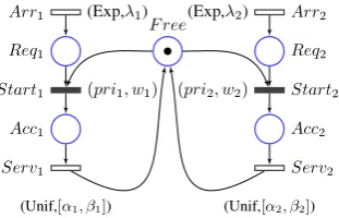
GSPN models. A GSPN model is a bipartite graph consisting of two classes of nodes:placesand transitions. Places may

containtokens(representing the state of the modelled system) while transitions indicate how tokens ‘‘flow’’ within the net (encoding the model dynamics). The state of a GSPN consists of amarkingindicating the distribution of tokens among the places (i.e. how many tokens each place contains). Roughly speaking a transitiont is enabled whenever everyinput placeoftcontains a number of tokens greater than or equal to the multiplicity of the corresponding (input) arc. An enabled transition mayfire, consuming tokens (in a number indicated by the multiplicity of the corresponding input arcs) from its input places, and producing tokens (in a number indicated by the multiplicity of the corresponding output arcs) in its output places. Transitions can be eithertimed(denoted by empty bars) orimmediate(denoted by filled-in bars, seeFig. 1). Transitions are characterised by: (1) adistributionwhich randomly determines the delay before firing it; (2) apriority which deterministically selects among the transitions scheduled the soonest, the one to be fired; (3) aweight, that is used in the random choice between transitions scheduled the soonest with the same highest priority. With the original GSPN formalism [12] the delay of timed transitions is assumedexponentiallydistributed, whereas with our GSPN it can be given by any distribution. Thus a GSPN timed-transition is characterised by a tuple:t

≡

(

type

,

par

,

pri

, w)

, wheretypeindicates the type of distribution (e.g. uniform),par indicates the parameters of the distribution (e.g.

[

α, β

]

),pri

∈

R+_{is a priority}

assigned to the transition and

w

∈

R+_{is used to probabilistically choose between transitions occurring with equal delay}

and equal priority. Observe that the information associated with a transition (i.e.type

,

par

,

pri

, w

) is exploited in different manners depending on the type of transition. For example for a transition with a continuous distribution the priority (pri) and weight (

w

) records are superfluous (hence ignored) since the probability that the schedule of the corresponding event is equal to the schedule of the event corresponding to another transition is null. Similarly, for an immediate transition (denoted by a filled-in bar) the specification of the distribution type (i.e.type) and associated parameters (par) is irrelevant (hence also ignored). Therefore these unnecessary informations are omitted inFig. 1.

Running example. This model will be used in Section3for describing, through a couple of LHA examples, the intuition behind hybrid automata based verification. We consider the GSPN model ofFig. 1(inspired by [12]). It describes the behaviour of an open system where two classes of clients (processes) (namely 1 and 2) compete to access a shared resource (memory). Class i-clients (i

∈ {

1

,

2

}

) enter the system according to a Poisson process with parameter

λ

i(corresponding to the exponentially

distributed timed transitionArriwith rate

λ

i). On arrival, clients cumulate in placesReqiwaiting for the resource to be free

(a token in placeFreewitnessing that the resource is available). The exclusive access to the shared resource is regulated either deterministically or probabilistically by thepriority(prii) and theweight (

w

i) of immediate transitionsStart1and

Start2. Thus in presence of a competition (i.e. one or more tokens in bothReq1andReq2) a classiclient wins the competition

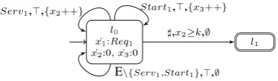
Fig. 2. An LHA to compute the bounds on the waiting time.

time of the resource by a classiclient is assumed to be uniformly distributed within the interval

[

α

i

, β

i

]

(corresponding to

transitionsServi). Thus on firing transitionServithe resource is released and a classiclient leaves the system.

3. HASL

The use of statistical methods instead of numerical ones gives us the possibility to relieve the limitations that were inherent to numerical methods, in terms of model and properties. When numerical model checking was focusing on Markovian models, statistical methods permit to use a very wide range of distributions, and tosynchronisesuch a model with an automaton that includes linearly evolving variables, complex updates and constraints. We are no more limited to the probability with which a property is satisfied, we can also compute the expected value of performability parameters such as waiting time, number of clients in a system, production cost of an item. In this section, we present the Hybrid Automata Stochastic Language, first introduced in [5], and illustrate its expressiveness on examples. We intuitively describe the syntax and semantics of HASL before formally defining them in the next subsections. A formula of HASL consists of two parts:

•

The first component of a formula is a hybrid automaton that synchronises with an infinite timed execution of the considered DESP until some final location is reached (i.e. the execution is successful) or the synchronisation fails. This automaton uses data variables evolving along the path. They both enable to select the subset of successful executions and maintain detailed information on the path.

•

The second component of a formula is an expression based on the data variables that expresses the quantity to be evaluated. In order to express path indices, they include path operators such as min and max values along an execution, value at the end of a path, integral over time and the time average value operator. Conditional expectations over the successful paths are applied to these indices in order to obtain the value of the formula.2

In order to illustrate our formalism, we consider the automaton ofFig. 2. Its purpose is to compute the lower and upper bounds on the waiting time for clients of type 1 in the DESP ofFig. 1. It has three data variables, whose evolution rate is indicated in locationl0. Variablex2(resp.x3) is a counter to record the number of completed (resp. started) accesses of type

1 clients to the shared resource. Variablex1counts the cumulated waiting time for all clients of type 1, thus the rate ofx1in

locationl0is equal to the number of type 1 clients waiting for the resource (Req1). The transitions can either be synchronised

and triggered by the actions of the DESP (the self loops) whereServ1(resp.Start1) denotes the end (resp. beginning) of

type 1 service, or autonomous (denoted by

♯

) and triggered by the evolution of the variables’ values (transition to the final locationl1).

An execution of this automaton terminates in final locationl1afterktype 1 clients have completed their access to the

shared resource. The formulas used to compute the aforementioned bounds are presented in Section3.2. Let us explain the behaviour of the synchronised product of the LHA and the DESP, based on the following execution withk

=

1. Initially in the DESP two transitions (Arr1andArr2) are enabled and so (randomly) scheduled respectively at times 3 and 17. The

LHA starts in locationl0 with all variables initialised to 0. Since the rate ofx2in l0 is null, the autonomous transition

labelled by

♯

and guarded byx2

≥

1 cannot be eventually fired. So the initial state of this execution is:

((

Free

,

0

, (

Arr1

:

3

,

Arr2

:

17

)), (

l0

, (

0

,

0

,

0

)))

where the first component of this couple is the marking of the GSPN, the current time, and

the time schedules of its enabled transitions while the second component is the location of the LHA and the values of its data variables. Then transitionArr1is fired synchronising with the loop belowl0.Start1is now enabled and is scheduled

immediately (due to its Dirac distribution). In addition,Arr1is again enabled and scheduled (at time 12). This leads to:

((

Req1

+

Free

,

3

, (

Arr1

:

12

,

Arr2

:

17

,

Start1

:

3

)), (

l0

, (

0

,

0

,

0

)))

. The firing ofStart1is synchronised with the upper right

loop incrementingx3. This leads to:

((

Acc1

,

3

, (

Arr1

:

12

,

Arr2

:

17

,

Serv1

:

15

)), (

l0

, (

0

,

0

,

1

)))

. A new client of type 1 arrives

at time 12, with the scheduling of a new client at time 20:

((

Req₁

+

Acc1

,

12

, (

Arr1

:

20

,

Arr2

:

17

,

Serv1

:

15

)), (

l0

, (

0

,

0

,

1

)))

.

When the first client is served at time 15, this leads to a synchronisation with the upper left loop andx2is incremented. In

addition the rate ofx1is 1, and so at the time of the firingx1is incremented by 3:

((

Req1

+

Free

,

15

, (

Arr1

:

20

,

Arr2

:

17

,

Start1

:

15

, ♯

:

15

)), (

l0

, (

3

,

1

,

1

)))

. Observe that the autonomous transition and a synchronised one are scheduled at

the same time (15). Since an autonomous transition has higher priority, it is fired. The resulting location is a final one and so the reached state is an absorbing state of the product:

((

Req1

+

Free

,

15

), (

l1

, (

3

,

1

,

1

)))

.

We will now proceed to a more formal definition of the automata and expressions used in HASL.

3.1. Synchronised Linear Hybrid Automata

Syntax. The first component of a HASL formula is a restriction of a hybrid automaton [14], namely a synchronised Linear Hybrid Automaton (LHA). Such automata extend the Deterministic Timed Automata (DTA) used to describe properties of Markov chain models [6,7]. Simply speaking, LHA are automata whose set oflocationsis associated with an-tuple of real-valued variables (called data variables) whose rate can vary.

In our context, the LHA is used to synchronise with DESP paths. However, it can evolve in an autonomous way. The symbol

♯

, associated with these autonomous changes, is thus used to denote a pseudo-event that is not included in the event setE of the DESP. The transitions in the synchronised system (DESP

+

LHA) are either autonomous,i.e.time-triggered (or rather variable-triggered) and take place as soon as a constraint is satisfied, or synchronisedi.e.triggered by the DESP and take place when an event occurs in the DESP. The LHA will thus take into account the system behaviour through synchronised transitions, but also take its own autonomous transitions in order to evaluate the desired property.

The values of the data variablesx1

, . . . ,

xnevolve with a linear rate depending both on the location of the automaton and

on the current state of the DESP. More precisely, the functionflowassociates with each location of the automaton ann-tuple of indicators (one for each variable) and, given a statesof a DESP and a locationl, the flow of variablexiin

(

s

,

l

)

isflowi

(

l

)(

s

)

(whereflowi

(

l

)

is theith component offlow

(

l

)

). Our model also usesconstraints, which describe the conditions for an edge

to be traversed, andupdates, which describe the actions taken on the data variables on traversing an edge. Aconstraintof an LHA edge is a boolean combination of inequalities of the form



1≤i≤n

α

ixi

+

c

≺

0 where

α

i

,

c

∈

Indare indicators,

and

≺∈ {=

, <, >,

≤

,

≥}

. The set of constraints is denoted byConst. Given a location and a state, an expression of the

form



1≤i≤n

α

ixi

+

clinearly evolves with time. An inequality thus gives an interval of time during which the constraint is

satisfied. We say that a constraint is left closed if, whatever the current statesof the DESP (defining the values of indicators), the time at which the constraint is satisfied is a union of left closed intervals. These special constraints are used for the ‘‘autonomous’’ edges, to ensure that the first time instant at which they are satisfied exists. We denote bylConstthe set of left closed constraints.

Anupdateis more general than the reset of timed automata. Here each data variable can be set to a linear function of the variables’ values. An updateUis then ann-tuple of functionsu1

, . . . ,

unwhere eachukis of the formxk

=



1≤i≤n

α

ixi

+

c

where the

α

iandcare indicators. The set of updates is denoted byUp.

Definition 2. Asynchronised linear hybrid automaton (LHA) is defined by a tupleA

= ⟨

E

,

L

,

Λ

,

Init

,

Final

,

X

,

flow

,

→⟩

where:

•

Eis a finite alphabet of events;

•

Lis a finite set of locations;

•

Λ

:

L

→

Propis a location labelling function;

•

Initis a subset ofLcalled the initial locations;

•

Finalis a subset ofLcalled the final locations;

•

X

=

(

x1

, . . . ,

xn

)

is an-tuple of data variables;

•

flow

:

L

→

Indn_{is a function which associates with each location one indicator per data variable representing the}

evolution rate of the variable in this location.flowidenotes the projection offlowon itsith component.

•

The transition relation

→⊆

L

×



•

No

♯

-labelled loops: For all sequences

l0

E0,γ0,U0

−−−−→

l1

E1,γ1,U1

−−−−→ · · ·

−−−−−−−−→

En−1,γn−1,Un−1 lnsuch thatl0

=

ln, there existsi

≤

nsuch thatEi

̸=

♯

.

Illustration. In order to make this definition more concrete, we get back to the automaton ofFig. 2. On this automaton the set of eventsEisArri

,

StartiandServiwithi

∈ {

1

,

2

}

corresponding to the events of the associated GSPN ofFig. 1. The setL

of locations consists ofl0andl1. Locationl0is initial and locationl1is final. There are no labelling functions (such asacc1, noaccandacc2which can be found inFig. 3). The set of data variables isX

= {

x0

,

x1

,

x2

}

. Concerning the flow, the last

two variables have rate 0 inl0whereasx0evolves with a rate that is equal to the marking of placeReq1inFig. 1. The rate

loop onl0is triggered as soon as actionServ1is fired in the GSPN, it has trivial constraint

⊤

(True) and its update consists in

incrementingx2. The transition froml0tol1is not synchronised (label

♯

), has a left closed constraintx2

≥

kand no update.

Discussion. The automata we consider are deterministic in the following (non usual) sense. Given a path

σ

of a DESP, there is at most one synchronisation with the linear hybrid automaton. The three first constraints ensure that the synchronised system is still a stochastic process. The fourth condition disables ‘‘divergence’’ of the synchronised product, i.e. the possibility of an infinity of consecutive autonomous events without synchronisation.

It should also be said that the restriction to linear equations in the constraints and to a linear evolution of data variables can be relaxed, as long as they are not involved in autonomous transitions. Polynomial evolution of constraints could easily be allowed for synchronised edges for which we would just need to evaluate the expression at a given time instant. Since the best algorithms solving polynomial equations operate in PSPACE [15], such an extension for autonomous transitions cannot be considered for obvious efficiency reasons.

Notations. Avaluation

ν

:

X

→

R_{maps every data variable to a real value. In the following, we useValto denote the set}

of all possible valuations. The value of data variablexi in

ν

is denoted

ν(

xi

)

. Let us fix a valuation

ν

and a states. Given

an expressionexp

=



Semantics. The role of a synchronised LHA is, given an execution of a corresponding DESP, to decide whether the execution is to be accepted or not, and also to maintain data values along the execution. Before defining the model associated with the synchronisation of a DESPD_{and an LHA}A_{, we need to introduce a few notations to characterise the evolution of a}

synchronised LHA. Given a statesof the DESP, a non final locationland a valuation

ν

ofA_{, we define the effect of time}

elapsing by:Elapse

(

s

,

l

, ν, δ)

=

ν

′where, for every variablexk,

ν

′

(

xk

)

=

ν(

xk

)

+

flowk

(

l

)(

s

)

×

δ

. We also introduce the

autonomous delayAutdel

(

s

,

l

, ν)

:

Autdel

(

s

,

l

, ν)

=

min

(δ

| ∃

l

−

♯,γ ,

−−

→

U l′

∧

s

|=

Λ

(

l′

)

∧

(

Elapse

(

s

,

l

, ν, δ))

|=

γ ).

WheneverAutdel

(

s

,

l

, ν)

is finite, we know that there is at least one executable transition with minimal delay and, thanks to the ‘‘determinism on

♯

’’ ofDefinition 2, we know that this transition is unique. In the following we denoteNext

(

s

,

l

, ν)

the target location of this first transition andUmin

(

s

,

l

, ν)

its update. We now proceed to the formal definition of the DESP,

D′

_{= ⟨}

_S′

_{, π}

′

Note that this definition gives a distribution since, due to ‘‘initial determinism’’ ofDefinition 2, for everys

∈

S, there is at most onel

∈

Initsuch thats

|=

Λ

(

l

)

.

•

E′

₌

_E

_{⊎ {}

_♯

_}

•

Ind′

_{= ∅}

_{. In factInd}′_{is useless since there is no more synchronisation to make.}

•

ifAutdel

(

s

,

l

, ν)

̸= ∞

then

Due to the determinism, there is at most one such transition.

•

For an autonomous event

♯

∈

enabled′

₍

_s

_,

_l

_{, ν),}

_target′

₍₍

_s

_,

_l

_{, ν), ♯)}

₌

₍

_s

_,

_l′

_{, ν}

′

₎

_withl′

₌

_Next

₍

_s

_,

_l

_{, ν)}

_and

ν

′

₌

_Umin

₍

_s

_,

_l

_{, ν)(}

_Elapse

₍

_s

_,

_l

_{, ν,}

_Autdel

₍

_s

_,

_l

_{, ν)))}

_.

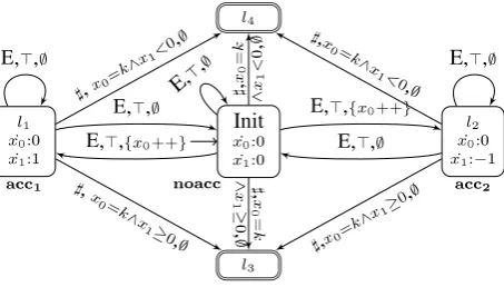
Fig. 3. An LHA to compute the difference of shared resource usage.

Fig. 4. An LHA for experimentφ3of FMS case study (Section5.1).

Roughly speaking, as long as the automaton is not in a final state, the product of a DESP and an LHA waits for the first transition to occur. If it is an autonomous one then only the location of the automaton and the valuation of variables change. If it is a synchronised event triggered by the DESP, either the LHA can take a corresponding transition and the system goes on with the next transition or the system goes to a dedicated rejecting state

⊥

implying the immediate end of the synchronisation. In case of a conflict of two transitions, an autonomous and a synchronised one, the autonomous transition is taken first.

Note that, by initial determinism, for everys

∈

Sthere is at most onel

∈

Initsuch thatssatisfiesΛ

(

l

)

. In case there is no suchlthe synchronisation starts and immediately ends up in the additional state

⊥

. Determinism on events (resp.on

♯

) ensures that there is always at most one synchronised (resp.autonomous) transition fireable at a given instant.

Example. The three LHAs ofFigs. 2–4intend to illustrate the expressiveness of LHAs in the context of HASL. When the first two are meant to synchronise with the shared resource system ofFig. 1, the last one expresses a property of the flexible manufacturing systems presented inFig. 8. Note that in the LHAs presented hereinafter,

♯

labels for autonomous transitions are omitted; furthermore, labelEis used to denoteuniversalsynchronisation (i.e. synchronisation with any event). The example ofFig. 2uses indicator dependent flows and has already been explained in the beginning of Section3.

The LHA in Fig. 3illustrates the interest of associating state propositions with locations of the LHA (functionΛof

Definition 2). In the figure, three such propositions are used, associated to non final locations:acc1(there is a token in placeAcc1),acc2(there is a token in placeAcc2) andnoacc(there is no token neither inAcc1nor inAcc2). The interest of

such propositions is that the automaton can take a transition to locationl1only ifacc1has value 1 in the corresponding state of the system. Hence, starting from locationInit, no matter which precise event occurs in the system, the automaton will switch fromInittol1andl2depending on which class of clients has access to the resource. The fact that for example three

different transitions labelled withEwithout any constraint are available in locationInitdoes not induce nondeterminism as only one of these transitions is possible at a time thanks to the state propositions. The automaton uses variablesx0that

is used to count the number of granted resource accesses andx1that expresses the difference of resource usage between

clients of class 1 and 2. To do so variablex1has flow 1 (resp.-1) when the resource is used by class 1 (resp.2) clients, and

0 when the resource is not used. In figures, we denote the flow of variablexbyx. As soon as

˙

kclients have been given a resource access, the system terminates in locationl3orl4depending on which client type has used the resource for the

longest cumulated period.

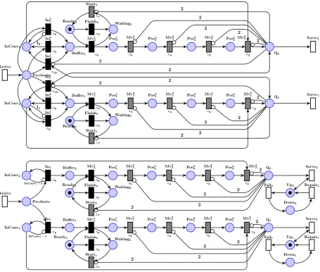
The LHA ofFig. 4is meant to compute the probability to have at leastKproduct completions (events corresponding to transitionsServ1andServ2of the FMS Petri nets of Section5) in a time interval of durationDduring horizonmD. The three

variables represent respectively the total time (x1), the time and the number of product completions since the beginning of

the interval (x2andx3). The automaton reaches a final state when the time horizon is reached (statel1). The value ofx4at

3.2. HASL expressions

The second component of a HASL formula is an expression related to the automaton. Such an expression, denotedZ, is based on moments of a path random variableYand defined by the grammar:

Z

::=

c

|

P

|

E

_[

_Y

_]|

_Z

₊

_Z

_|

_Z

₋

_Z

_|

_Z

_×

_Z

_|

_Z

_/

_Z

Y

::=

c

|

Y

+

Y

|

Y

×

Y

|

Y

/

Y

|

LAST

(

y

)

|

MIN

(

y

)

|

MAX

(

y

)

|

INT

(

y

)

|

AVG

(

y

)

y

::=

c

|

x

|

y

+

y

|

y

×

y

|

y

/

y

(1)

Preliminary assumption. Before explaining this syntax, we emphasise that given an infinite path of the synchronised product, the formula is evaluated on the finite prefix that ends when the path reaches an absorbing state. In the general case, it would be possible that an infinite path does not admit such a prefix. Here we assume that given a DESPDand a HASL formula

(

A

_,

Z

)

, with probability 1, the synchronising path generated by a random execution path ofD_{reaches an absorbing configuration.}

This semantical assumption can be ensured by structural properties ofA_and/orD_{. For instance, the time bounded}

Until

of CSL guarantees this property. As a second example, the time unbounded

Until

_{of CSL also guarantees this property when}

applied on finite CTMCs where all terminal strongly connected components of the chain include a state that either fulfils the target sub-formula of the

Until

operator or falsifies the continuing sub formula. This (still open) issue is also addressed in [16,17].

The variableyis an arithmetic expression built on top of LHA data variables (x) and constants (c). A path variableY is a path dependent expression built on top of basic path random variables such asLAST

(

y

)

(i.e. the value ofywhen reaching the absorbing state),MIN

(

y

)

(resp.MAX

(

y

)

), the minimum (resp. maximum), value ofyalong a synchronising path,INT

(

y

)

(i.e. the integral over time along the finite prefix) andAVG

(

y

)

(the average value ofyalong a path). FinallyZ, the actual target of HASL verification, is eitherP, denoting the probability that a path is accepted by the LHA or an arithmetic expression. Such an expression is built on top of the first moment ofY (E

_[

_Y

_]

_{), and thus allowing for the consideration of} diverse significant characteristics ofY(apart from its expectation) as the quantity to be estimated, including, for example, the varianceVar

[

Y

] ≡

E

_[

_Y2

_{] −}

E

_[

_Y

_]

2_{and the covarianceCovar}

_[

_Y1

_,

_Y2

_{] ≡}

E

_[

_Y1Y2

_{] −}

E

_[

_Y1

_]

E

_[

_Y2

_]

_{. Note that for efficiency} reasons, in the implementation of the Cosmossoftware tool, we have considered a restricted version of grammar(1), where products and quotients of data variables (e.g.x1

×

x2andx1

/

x2) are allowed only within the scope of theLASToperator (i.e.

not withMIN

,

MAX

,

INTorAVG). Indeed, allowing products and quotients as arguments of path operators such asMAXor MINrequires the solution of a linear programming problem during the generation of a synchronisedD

_×

A_{path which,}

although feasible, would considerably affect the computation time.

Example. With the LHA ofFig. 2, we can express bounds for the average waiting time until the firstkclients have been served. The upper (resp. lower) bound on the waiting time is computed by the final value ofx1divided byk(resp.x3). In our

formalism it corresponds to the expressionsE

_[

_LAST

₍

_x1

_)/

_k

_]

_{for the upper bound and to}E

_[

_LAST

₍

_x1

_)/

_LAST

₍

_x3

₎

_]

_{for the lower} bound. Referring to the LHA ofFig. 3, we can consider path random variables such asY

=

LAST

(

x1

)

(the final difference of

shared resource usage), orY

=

AVG

(

x1

)

(the average along paths of such a difference). Furthermore, with a slight change of

the automaton (settingx0to 0 (resp.1) when reachingl4(resp. l3)),E

[

LAST

(

x0

)

]

will give the probability to reachl3. Finally,

on the LHA ofFig. 4, the ratio of time intervals of the form

[

nD

, (

n

+

1

)

D

[

during whichKproduct completions occur is evaluated through expressionE

_[

LAST

(

x4

)

]

.

Semantics. We emphasise that the (conditional) expectation of a path random variable is not always defined. There are two obvious necessary conditions on the synchronised product: (1) almost surely the random execution ends either in a final state of the LHA or in the rejecting state, and (2) with positive probability the random execution ends in a final state of the LHA. However these conditions are not sufficient. Different restrictions on the path formula ensure the existence of expectations. For instance, when the formula only includes bounded data variables and the operatorINTand the division are excluded, the expectation exists. Divisions may be allowed when the path expression is lower bounded by a positive value: in the example ofFig. 2,LAST

(

x3

)

is lower bounded byLAST

(

x2

)

which is lower bounded byk. The existence of regeneration

points of the synchronised product may also entail the existence of such expectations. We do not detail the numerous possible sufficient conditions but in all considered applications here, it can be proved that the expectations exist.

3.3. Expressiveness of HASL

In this subsection we first give an overview of related logics. Then we discuss the expressiveness of HASL and show how it improves the existing formalisms to capture more complex examples and properties, and facilitates the expression and the computation of costs and rewards.

CSL and its variants. In [4] Continuous Stochastic Logic (CSL) has been introduced and the decidability of the verification problem over a finite continuous-time Markov chain (CTMC) has been established. CSL extends thebranching timereasoning of CTL to CTMC models by replacing the discrete CTL path-quantifiers

All

_and

Exists

_{with a continuous path-quantifier}

the

Until

or

Next

operator. asCSL, introduced in [19] replaces the interval time constrained

Until

of CSL by a regular expression with a time interval constraint. These path formulas can express elaborated functional requirements as in CTL∗ but the timing requirements are still limited to a single interval globally constraining the path execution. In the logic CSLTA[6], path formulas are defined by a single-clock deterministic timed automaton. This logic has been shown strictly more expressive than CSL and also more expressive than asCSL when restricted to path formulas.

DTA. In [7], deterministic timed automata with multiple clocks are considered and the probability for random paths of a CTMC to satisfy a formula is shown to be the least solution of a system of integral equations. The cost of this more expressive model is both a jump in the complexity as it requires to solve a system of partial differential equations, and a loss in guaranty on the error bound.

M(I)TL. Several logics based on linear temporal logic (LTL) have been introduced to consider timed properties, including Metric (Interval) Temporal logic in which the

Until

operator is equipped with a time interval. Chen et al. [20] have designed procedures to approximately compute desired probabilities for time bounded verification, but with complexity issues. The question of stochastic model checking on (a sublogic of) M(I)TL properties, has also been tackled see e.g. [21].

Observe that all of the above mentioned logics have been designed so that numerical methods can be employed to decide about the probability measure of a formula. This very constraint is at the basis of their limited expressive scope which has two aspects: first the targeted stochastic models are necessarily CTMCs; second the expressiveness of formulas is constrained by decidability/complexity issues. Furthermore the evolution of stochastic logics based on CTL seems to have followed two directions: one targetingtemporal reasoning capability (in that respect the evolutionary pattern is: CSL

→

asCSL

→

CSLTA

→

DTA), the other targetingperformance evaluationcapability (evolutionary path: CSL

→

CSRL

→

CSRL

+

impulse rewards). A unifying approach is currently not available, thus, for example, one can calculate the probability for a CTMC to satisfy a sophisticated temporal condition expressed with a DTA, but cannot, assess performance evaluation queries at the same time (i.e. with the same formalism).

HASL. As HASL is inherently based on simulation for assessing measures of a model, it naturally allows for releasing the constraints imposed by logics that rely on numerical solution of stochastic models. From a modelling point of view, HASL allows for studying a broad class of stochastic models (i.e. DESP), which includes, but is not limited to, CTMCs. From an expressiveness point of view, the use of LHAs allows for generic variables, which include, but are not limited to, clock variables (as per DTA). This means that sophisticated temporal conditions as well as elaborate performance measures of a model can be accounted for in a single HASL formula, rendering HASL a unified framework suitable for both model-checking and performance and dependability studies. Note that the nature of the (real-valued) expressionZ, available in grammar

(1), generalises the common approach of stochastic model checking where the outcome of verification is (an approximation of) the mean value of a certain measure (with CSL, asCSL, CSLTAand DTA a measure of probability).

It is also worth noting that the use of data variables and extended updates in the LHA enables to compute costs/rewards naturally. The rewards can be both on locations and on actions. First using an appropriate flow in each location of the LHA, possibly depending on the current state of the DESP we get ‘‘state rewards’’. Then, by considering theupdate expressionson the edges of the LHA, we can model sophisticated ‘‘action rewards’’ that can either be a constant, depend on the state of the DESP and/or depend on the values of the variables. Thus HASL extends the possibilities of CSRL (and extensions [18]). The extension does not only consist of the possibility to define multiple rewards (that can be handled, for example, through the reward-enriched version of CSL supported by the PRISM [22] tool) but rather of their use. First several rewards can be used in the same formula, and last but not least these rewards have a more active role, as they can not only be evaluated at the end of the path, but they can also take an important part in the selection of enabled transitions, hence of accepted paths. It is for example possible and easy to characterise the set of paths along which a reward reaches a given value and after that never goes below another value, a typical example that neither PRISM–CSL nor CSRL can handle.

Limitations of HASL. Finally, we briefly discuss two features that are available in the above mentioned stochastic logics but not in HASL. First HASL does not allow to properly model nesting of probabilistic operators. The key reason is that this nesting is meaningful only when an identification can be made between a state of the probabilistic system and a configuration (comprising the current time and the next scheduled events). While this identification was natural for Markov chains, it is not possible with DESP and general distributions that have no memoryless property, and therefore this operation has not been considered in HASL. Furthermore, even for Markovian systems, the complexity of the statistical method on formulas with nesting is quite high [3] as the verification time per state along a path is no longer constant.

A similar problem arises for the steady state operator. The existence of a steady state distribution raises theoretical problems, except for finite Markov chains. With HASL we allow for not only infinite state systems but also non Markovian behaviours. However, when the DESP has a regeneration point, various steady state properties can be computed considering the sub-execution between regeneration points.

Proposition 1. Given a non nested transient CSRL formula P◃▹q

φ

and a system described as a Markov Reward Model, it is possible

to build an LHA to estimate the probability p for

φ

to hold, and then decide whether it fulfils the bound required (i.e. p

◃▹

q with

◃▹∈ {

<, >,

≤

,

≥}

).

To prove this proposition, we first need to characterise what is a non nested transient CSRL formula. Following the grammar given in [8], such a formula is either a boolean combination of atomic propositions, or of the formP◃▹qXJI

ϕ

orP◃▹q

ϕ

UIJ

ψ

with

ϕ

and

ψ

being boolean combinations of atomic propositions. Roughly speaking, path formulaXI

J

ϕ

means that the first

transition in the system will occur after a time delay in intervalIand accumulated reward within intervalJ, and that it will lead to a state satisfying

ϕ

. The second path formula

ϕ

UI_J

_ψ

means that the path reaches, with a delay inIand a cumulated reward inJa state satisfying

ψ

, and that all preceding states satisfy

ϕ

. The case of boolean formulas being rather trivial, we will focus onP◃▹qXJIandP◃▹qUIJ.

The kind of systems on which CSRL formulas are checked is called Markov Reward Model (MRM), which consists of a finite state labelled continuous time Markov chain plus two reward structures: one on actions and one on states. In our formalism, the MRM will be represented by both a GSPN and an LHA. The underlying labelled Markov chain will be represented by a GSPN. For each statesiof the MRM we create one placePiof the GSPN, and an indicatorpithat is true when a token is in

placePi, and for every couple of states

(

si

,

sj

)

such that the rate in the MRM isR

(

si

,

sj

)

=

rij

>

0, we add a transitiontijwith

input placePi, output placePjand exponential distribution using raterij. The atomic propositions of the MRM are simply

encoded as indicators, now on places instead of states.

For a formula of the kindP◃▹qXJI

ϕ

the LHA is quite simple. First the boolean formula

ϕ

is transformed straightforwardly

into a state propositionpϕon the GSPN. It has one initial locationInitiper statesiof the MRM, plus two final locations, one

calledf1labelled withpϕ, the otherf2with

¬

pϕ. It also has three data variables,twith rate 1 in every location for the global time,OK with rate 0 in every location to determine whether an execution satisfies the property or not, andrto capture the reward structure. In order to ensure initial determinism (seeDefinition 2), eachInitjis labelled with indicatorpj. The

reward structure is captured by a data variablerwhose rate inInitiis

ρ(

si

)

, the reward on statesiin the MRM. Then, for

every transition

(

si

,

sj

)

with impulse reward

ι(

si

,

sj

)

of the MRM, the LHA has three transitions starting fromIniti. The first

one, taken if statesjof the MRM does not satisfy

ϕ

, setsOK to 0 and leads to locationf2. The two other transitions lead to

f1and setOKto 1 or 0 depending on whether the interval constraintc

=

t

∈

I

∧

r

+

ι(

si

,

sj

)

∈

Jis satisfied or not. The

probability to satisfyX_JI

ϕ

is computed by the expressionE

_[

_LAST

₍

_OK

₎

_]

_{that can then be compared to boundq.}

As for

Until

operator, it is also possible to build an LHA to compute the desired probability, but this automaton is more complicated. In order not to make this part too long, we just give here an idea of the LHA checking

Until

formulas. It is again built based on the corresponding MRM. First, if the value 0 is not both inIandJ, for the states satisfying

¬

ϕ

the synchronisation ends immediately settingOKto 0. If 0 belongs to both intervals then, starting in a state satisfying

¬

ϕ

∧

ψ

, the synchronisation immediately ends settingOKto 1. For all other states of the MRM we create a corresponding location in the LHA from which we will follow the evolution of the MRM (with rates on locations modelling the state rewards and updates modelling the impulse rewards). A further distinction has to be made between locations satisfying both

ϕ

and

ψ

and others. Indeed, in the first case, time can pass without further transition of the GSPN and the formula become true. This has to be detected. Otherwise, the transitions will then synchronise with those of the GSPN and check whether time and reward after the MRM transition are within the interval bounds. If yes then the execution will either end if

ψ

is satisfied or if neither

ϕ

nor

ψ

are, settingOKto 1 and 0 respectively, or go on until the above solution occurs. If time or reward passes over its interval, the synchronisation ends settingOKto 0. In all other cases the synchronisation goes on.

On the automata built according to the above described method, the desired probability can then be computed using again expressionE

_[

_LAST

₍

_OK

₎

_]

_{and compared to the desired bound}

Proposition 2. Given a non nested transientCSLTAformula P◃▹qA

(φ

1

, . . . , φ

n

)

and a system described as a Continuous Time

Markov Chain, it is possible to build an LHA to estimate the probability p for an execution to be accepted by the DTAA

_(φ

₁

_{, . . . , φ}

_n

₎

_,

and then decide whether it fulfils the bound required (i.e. p

◃▹

q with

◃▹ ∈ {

<, >,

≤

,

≥}

).

Since DTA is a class of automata that is a strict subset of LHA, the construction is rather simple since the DTA can itself be used. It however has to be slightly modified. Indeed, the DTA was rejecting executions not satisfying the property. For the LHA we need to accept all executions and add a variable OK that is set to 0 or 1 depending whether the execution satisfies the desired property. Thus all transitions leading to an accepting location are enriched with the update OK

:=

1. Furthermore, for every location of the automaton we add transitions setting OK to 0 and leading to a new accepting location KO to ensure that every transition of the GSPN can synchronise with the LHA. For example in a location with a single outgoing transition labellede

,

x

≤

a

,

∅

we add two transitions to KO with labelE

\{

e

}

,

true

,

OK

:=

0 ande

,

x

>

a

,

OK

:=

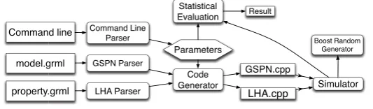
0.

4. Software support

In order to provide a software support to the HASL formalism we developed Cosmos3[9], a prototype software platform for HASL-based verification. In this section, we describe the Cosmos tool including its architecture and providing as