cover
n e x t pa ge >
title : Petroleum Processing Handbook
author : McKetta, John J.
publisher : CRC Press
isbn10 | asin : 0824786815
print isbn13 : 9780824786816
ebook isbn13 : 9780585375700
language : English
subject Petroleum--Refining--Handbooks, manuals, etc.
publication date : 1992
lcc : TP690.P4723 1992eb
ddc : 665.5/ 3
subject : Petroleum--Refining--Handbooks, manuals, etc.
Petroleum Processing Handbook
edited by John J. McKetta
The University of Texas at Austin Austin, Texas
< pr e viou s pa ge
page_ii
n e x t pa ge >
Page iiLibrary of Congress Cataloging-in-Publication Data
Petroleum processing handbook / edited by John J. McKetta. p. cm.
"The contents of this volume were originally published in Encyclopedia of chemical processing and design, edited by J.J. McKetta and W.A. Cunningham"-T.p. verso.
Includes bibliographical refernces and index. ISBN 0824786815 (alk. paper)
1. PetroleumRefiningHandbooks, manuals, etc. I. McKetta, John J. II. Encyclopedia of chemical processing and design. TP690.P4723 1992
665 .5′3-dc20 924374 CIP
The contents of this volume were originally published in Encyclopedia of Chemical Processing and Design, edited by J.
J. McKetta and W. A. Cunningham. © 1979, 1981, 1982, 1987, 1988, 1990 by Marcel Dekker, Inc. This book is printed on acid-free paper.
Copyright © 1992 by Marcel Dekker, Inc. All Rights Reserved.
Neither this book nor any part may be reproduced or transmitted in any form or by any means, electronic or mechanical, including photocopying, micro-filming, and recording, or by any information storage and retrieval system, without permission in writing from the publisher.
Marcel Dekker, Inc.
270 Madison Avenue, New York, New York 10016 Current printing (last digit):
10 9 8 7 6 5 4 3 2 1
PRINTED IN THE UNITED STATES OF AMERICA
PREFACE
It is time that many of the petroleum processes currently in use be presented in a well-organized, easy-to-read and understandable manner. This hand-book fulfills this need by covering up-to-date processing operations. Each chapter is written by a world expert in that particular area, in such a manner that it is easily understood and applied. Each
professional practicing engineer or industrial chemist involved in petroleum processing should have a copy of this book on his or her working shelf.
The handbook is conveniently divided into four sections: products, refining, manufacturing processes, and treating processes. Each of the processing chapters contain information on plant design as well as significant chemical reactions. Wherever possible, shortcut methods of calculations are included along with nomographic methods of solution. In the front of the book are two convenient sections that will be very helpful to the reader. These are (1) conversion to and from SI units, and (2) cost indexes that will enable the reader to update any cost information.
As Editor, I am grateful for all the help I have received from the great number of authors who have contributed to this book. I am also grateful to the huge number of readers who have written to me with suggestions of topics to be included.
JOHN J. MCKETTA
< pr e viou s pa ge
page_v
n e x t pa ge >
Bringing Costs up to Date xiii
1
John J. Lipinski and Jack R. Wilcox
25
Octane Catalysts
John S. Magee, Bruce R. Mitchell, and James W. Moore
31
Octane Options
Joseph A. Weiszmann, James H. D'Auria, Frederick G. McWilliams, and Frederick M. Hibbs
50
2 Refining
Petroleum Processing
Harold L. Hoffman and John J. McKetta
67
Petroleum Refinery of the Future
D. B. Bartholic, A. M. Center, Brian R. Christian, and A. J. Suchanek
108
Petroleum Processes, Catalyst Usage
Richard A. Corbett
130
Petroleum Processing Economics, Catalysts
Mattheus M. van Kessel, R. H. van Dongen, and G. M. A. Chevalier
155
Petroleum Refinery Yields Improvement
Dale R. Simbeck and Frank E. Biasca
Petroleum Waste Toxicity, Prevention
Raymond C. Loehr
190
Petroleum Refining Processes, United States Capacities
Debra A. Gwyn
199
Petroleum Refining Processes, Worldwide Capacities
Debra A. Gwyn
214
< pr e viou s pa ge
page_vi
n e x t pa ge >
W. P. Ballard, G. I. Cottington, and T. A. Cooper
281
Cracking, Catalytic
E. C. Luckenbach, A. C. Worley, A. D. Reichle, and E. M. Gladrow
349
Carl Pei-Chi Chang and James R. Murphy
Desulfurization, Liquids, Petroleum Fractions
Robert J. Campagna, James A. Frayer, and Raynor T. Sebulsky
697
Desulfurizing Cracked Gasoline and Other Hydrocarbon Liquids by Caustic Soda Treating
K. E. Clonts and Ralph E. Maple
727
Doctor Sweetening
Kenneth M. Brown
736
Index 759
< pr e viou s pa ge
page_vii
n e x t pa ge >
Page viiCONTRIBUTORS
W. P. Ballard Manager, Port Arthur Research Laboratories (Retired), Texaco, Inc., Port Arthur, Texas D. B. Bartholic Engelhard Corporation, Specialty Chemicals Division, Menlo Park, Edison, New Jersey
Richard A. Bausell Safety Services Manager, Cities Service Research and Development Company, Tulsa, Oklahoma Fabio Bernasconi, Ph.D. Ambrosetti Group, Milan, Italy
Frank E. Biasca Manager, Process Technology, SFA Pacific, Inc., Mountain View, California
D. E. Blaser Engineering Associate, Exxon Engineering Petroleum Department, Exxon Research and Engineering Company, Florham Park, New Jersey
Kenneth M. Brown Director, Treating Services (Retired), UOP Process Division, Des Plaines, Illinois
Donald R. Burris Manager, Technical Advisory Division, C-E Natco Combustion Engineering, Inc., Denver, Colorado Robert J. Campagna Gulf Science and Technology Company, Pittsburgh, Pennsylvania
John Caspers Manager, LC-Fining Design, C-E Lummus Company, Bloomfield, New Jersey
A. M. Center Engelhard Corporation, Specialty Chemicals Division, Menlo Park, Edison, New Jersey Carl Pei-Chi Chang Process Manager, Refinery Process Division, Pullman Kellogg, Houston, Texas G. M. A. Chevalier Shell Internationale Petroleum, Maatschappij BV, The Hague, The Netherlands
Brian R. Christian Engelhard Corporation, Specialty Chemicals Division, Menlo Park, Edison, New Jersey K. E. Clonts Vice President, Technical, Merichem Company, Houston, Texas
T. A. Cooper Staff Coordinator-Strategic Planning, Texaco, Inc., White Plains, New York Richard A. Corbett, P.E. Refining/Petrochemical Editor, Oil & Gas Journal, Houston, Texas
G. I. Cottington Technologist, Port Arthur Research Laboratories, Texaco, Inc., Port Arthur, Texas James H. D'Auria Director, Process Development, UOP Inc., Des Plaines, Illinois
J. A. Feldman Senior Process Analysis Engineer (Retired), Applied Automation, Inc., Bartlesville, Oklahoma James A. Frayer Technical Consultant, Gulf Science and Technology Company, Pittsburgh, Pennsylvania
E. M. Gladrow Senior Research Associate, Exxon Research and Development Laboratories, Baton Rouge, Louisiana Debra A. Gwyn Director of Editorial Surveys, Oil & Gas Journal, Tulsa, Oklahoma
R. L. Hair Information Technology Planner, Phillips Petroleum Company, Bartlesville, Oklahoma J. D. Hargrove The British Petroleum Company Limited, Sunbury-on-Thames, Middlesex, England
Kenneth E. Hastings Vice President and Director of Research, Cities Service Research and Development Company, Tulsa, Oklahoma
Frederick M. Hibbs UOP Inc., Des Plaines, Illinois
Harold L. Hoffman Editor, Hydrocarbon Processing, Houston, Texas
John J. Lipinski Coastal Eagle Point Oil Company, Westville, New Jersey
Raymond C. Loehr, Ph.D. H. M. Acharty Centennial Chair and Professor, Environmental Engineering Program, University of Texas at Austin, Austin, Texas
E. C. Luckenbach E. & R. Luckenbach and Co., Mountainside, New Jersey
B. E. Lutter Engineering Director, Automation Group, Applied Automation/Hartman and Braun, Bartlesville, Oklahoma John S. Magee, Ph.D. Technical Director, Katalistiks International, a unit of UOP, Inc., Baltimore, Maryland
Ralph E. Maple Assistant General Manager, Process Technology Division, Merichem Company, Houston, Texas John J. McKetta, Ph.D., P.E. The Joe C. Walter Professor of Chemical Engineering, The University of Texas at Austin, Austin, Texas
J. D. McKinney Gulf Research and Development Company, Pittsburgh, Pennsylvania Frederick G. McWilliams UOP Inc., Des Plaines, Illinois
Alice Megna Project Manager, ERT Inc., Dallas, Texas
< pr e viou s pa ge
page_ix
n e x t pa ge >
Page ixBruce R. Mitchell (deceased) Katalistiks International, a unit of UOP, Inc., Baltimore, Maryland
James W. Moore Senior Research Supervisor, Katalistiks International, a unit of UOP, Inc., Baltimore, Maryland James R. Murphy Pullman Kellogg, Houston, Texas
David Olschewsky Project Manager, ERT Inc., Dallas, Texas
John D. Potts Manager of Research Staff, Cities Service Research and Development Company, Tulsa, Oklahoma A. D. Reichie Engineering Advisor, Exxon Research and Development Laboratories, Baton Rouge, Louisiana G. G. Scholten Managing Director, Edeleanu GmbH, Frankfurt am Main, Germany
Raynor T. Sebulsky General Manager-Products, Refining & Products Division, Gulf Science and Technology Company, Pittsburgh, Pennsylvania
Avilino Sequeira, Jr., P. E. Senior Technologies, Texaco, Inc., Port Arthur, Texas
Dale R. Simbeck Vice President Technology, SFA Pacific, Inc., Mountain View, California
A. J. Suchanek Engelhard Corporation, Specialty Chemicals Division, Menlo Park, Edison, New Jersey R. H. van Dongen Shell Internationale Petroleum, Maatschappij BV, The Hague, The Netherlands
Roger P. Van Driesen Manager, Petroleum and Coal Process Marketing, C-E Lummus Company, Bloomfield, New Jersey
Mattheus M. van Kessel Product Manager, Refinery Catalysts, SICC, London, United Kingdom Hervey H. Voge (deceased) Sebastopol, California
Guy E. Weismantel President, Weismantel International, Kingwood, Texas
Joseph A. Weiszmann Marketing Manager, Western U.S., UOP, Inc., Des Plaines, Illinois Jack R. Wilcox Harshaw/Filtrol Partnership, Los Angeles, California
A. C. Worley Senior Engineering Associate, Exxon Research and Engineering Company, Florham Park, New Jersey
CONVERSION TO SI UNITS
To convert from To Multiply by
acre square meter (m2) 4.046 × 10³
angstrom meter (m) 1.0 × 10¹⁰
are square meter (m2) 1.0 × 10²
atmosphere newton/square meter (N/m2) 1.013 × 10⁵
bar newton/square meter (N/m2) 1.0 × 10⁵
barrel (42 gallon) cubic meter (m3) 0.159
Btu (International Steam Table) joule (J) 1.055 × 10³
Btu (mean) joule (J) 1.056 × 10³
Btu (thermochemical) joule (J) 1.054 × 10³
bushel cubic meter (m3) 352 × 102
calorie (International Steam Table) joule (J) 4.187
calorie (mean) joule (J) 4.190
calorie (thermochemical) joule (J) 4.184
centimeter of mercury newton/square meter (N/m2) 1.333 × 10³
centimeter of water newton/square meter (N/m2) 98.06
cubit meter (m) 0.457
degree (angle) radian (rad) 1.745 × 10²
denier (international) kilogram/meter (kg/m) 1.0 × 10⁷
dram (avoirdupois) kilogram (kg) 1.772 × 10³
dram (U.S. fluid) cubic meter (m3) 3.697 × 10⁶
dyne newton (N) 1.0 × 10⁵
electron volt joule (J) 1.60 × 10¹⁹
erg joule (J) 1.0 × 10⁷
fluid ounce (U.S.) cubic meter (m3) 2.96 × 10⁵
foot meter (m) 0.305
furlong meter (m) 2.01 × 10²
gallon (U.S. dry) cubic meter (m3) 4.404 × 10³
gallon (U.S. liquid) cubic meter (m3) 3.785 × 10³
gill (U.S.) cubic meter (m3) 1.183 × 10⁴
grain kilogram (kg) 6.48 × 10⁵
gram kilogram (kg) 10 × 103
horsepower watt (W) 7.457 × 10²
horsepower (boiler) watt (W) 9.81 × 10³
horsepower (electric) watt (W) 7.46 × 10²
hundred weight (long) kilogram (kg) 50.80
hundred weight (short) kilogram (kg) 45.36
inch meter (m) 2.54 × 10²
inch mercury newton/square meter (N/m2) 3.386 × 10³
inch water newton/square meter (N/m2) 2.49 × 10²
kilogram force newton (N) 9.806
To convert from To Multiply by
kip newton (N) 4.45 × 10³
knot (international) meter/second (m/s) 0.5144
league (British nautical) meter (m) 5.559 × 10³
league (statute) meter (m) 4.83 × 10³
light year meter (m) 9.46 × 10¹⁵
liter cubic meter (m3) 0.001
micron meter (m) 1.0 × 10⁶
mil meter (m) 2.54 × 10⁶
mile (U.S. nautical) meter (m) 1.852 × 10³
mile (U.S. statute) meter (m) 1.609 × 10³
millibar newton/square meter (N/m2) 100.0
millimeter mercury newton/square meter (N/m2) 1.333 × 10²
oersted ampere/meter (A/m) 79.58
ounce force (avoirdupois) newton (N) 0.278
ounce mass (avoirdupois) kilogram (kg) 2.835 × 10²
ounce mass (troy) kilogram (kg) 3.11 × 10²
ounce (U.S. fluid) cubic meter (m3) 2.96 × 10⁵
pascal newton/square meter (N/m2) 1.0
peck (U.S.) cubic meter (m3) 8.81 × 10³
pennyweight kilogram (kg) 1.555 × 10³
pint (U.S. dry) cubic meter (m3) 5.506 × 10⁴
poise newton second/square meter (N s/m2) 0.10
pound force (avoirdupois) newton (N) 4.448
pound mass (avoirdupois) kilogram (kg) 0.4536
pound mass (troy) kilogram (kg) 0.373
poundal newton (N) 0.138
quart (U.S. dry) cubic meter (m3) 1.10 × 10³
quart (U.S. liquid) cubic meter (m3) 9.46 × 10⁴
rod meter (m) 5.03
roentgen coulomb/kilogram (c/kg) 2.579 × 10⁴
second (angle) radian (rad) 4.85 × 10⁶
section square meter (m2) 2.59 × 10⁶
slug kilogram (kg) 14.59
span meter (m) 0.229
stoke square meter/second (m2/s) 1.0 × 10⁴
ton (long) kilogram (kg) 1.016 × 10³
ton (metric) kilogram (kg) 1.0 × 10³
ton (short, 2000 pounds) kilogram (kg) 9.072 × 10²
torr newton/square meter (N/m2) 1.333 × 10²
yard meter (m) 0.914
BRINGING COSTS UP TO DATE
Cost escalation via inflation bears critically on estimates of plant costs. Historical costs of process plants are updated by means of an escalation factor. Several published cost indexes are widely used in the chemical process industries:
Nelson Cost Indexes (Oil and Gas J.), quarterly
Marshall and Swift (M&S) Equipment Cost Index, updated monthly CE Plant Cost Index (Chemical Engineering), updated monthly
ENR Construction Cost Index (Engineering News-Record), updated weekly
All of these indexes were developed with various elements such as material availability and labor productivity taken into account. However, the proportion allotted to each element differs with each index. The differences in overall results of each index are due to uneven price changes for each element. In other words, the total escalation derived by each index will vary because different bases are used. The engineer should become familiar with each index and its limitations before using it.
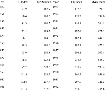
Table 1 compares the CE Plant Index with the M&S Equipment Cost
TABLE 1 Chemical Engineering and Marshall and Swift Plant and Equipment Cost
Indexes since 1950
Year CE Index M&S Index Year CE Index M&S Index
1962
102.0 238.5 1983 316.9 760.8
1963
102.4 239.2 1984 322.7 780.4
1964
103.3 241.8 1985 325.3 789.6
1965
104.2 244.9 1986 318.4 797.6
1966
107.2 252.5 1987 323.8 813.6
1967
109.7 262.9 1988 342.5 852.0
1968
113.6 273.1 1989 355.4 895.1
1969
119.0 285.0 1990 357.6 915.1
1970
125.7 303.3
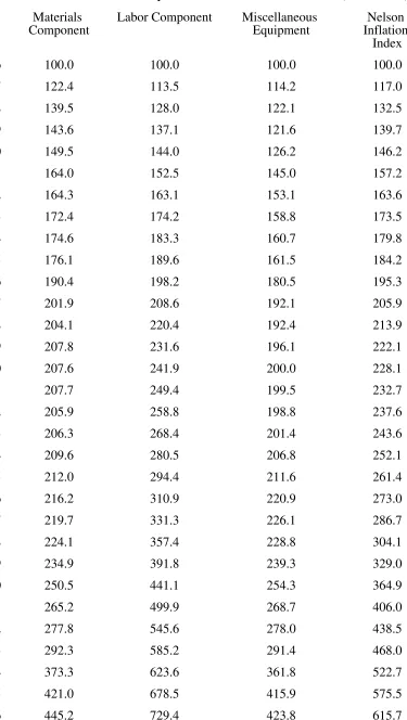
TABLE 2 Nelson Inflation Refinery Construction Indexes since 1946 (1946 = 100) Date Materials
1977 471.3 774.1 438.2 653.0
1978 516.7 824.1 474.1 701.1
1979 573.1 879.0 515.4 756.6
1980 629.2 951.9 578.1 822.8
1981 693.2 1044.2 647.9 903.8
1982 707.6 1154.2 622.8 976.9
1983 712.4 1234.8 656.8 1025.8
1984 735.3 1278.1 665.6 1061.0
1985 739.6 1297.6 673.4 1074.4
1986 730.0 1330.0 684.4 1089.9
1987 748.9 1370.0 703.1 1121.5
1988 802.8 1405.6 732.5 1164.5
1989 829.2 1440.4 769.9 1195.9
1990 832.8 1487.7 795.5 1225.7
Index. Table 2 shows the Nelson Inflation Petroleum Refinery Construction Indexes since 1946. It is recommeded that the CE Index be used for updating total plant costs, and the M&S Index or Nelson Index for updating equipment costs. The Nelson Indexes are better suited for petroleum refinery materials, labor, equipment, and general refinery inflation. Since
Here, A = the size of units for which the cost is known, expressed in terms of capacity, throughput, or volume; B = the
size of unit for which a cost is required, expressed in the units of A; n = 0.6 (i.e., the six-tenths exponent); CA = actual
cost of unit A; and CB = the cost for B being sought for the same time period as cost CA.
To approximate a current cost, multiply the old cost by the ratio of the current index value to the index at the date of the old cost:
Here, CA = old cost; IB = current index value; and IA = index value at the date of old cost.
Combining Eqs. (1) and (2):
For example, if the total investment cost of Plant A was $25,000,000 for 200-million-lb/yr capacity in 1974, find the
cost of Plant B at a throughput of 300 million lb/yr on the same basis for 1986. Let the sizing exponent, n, be equal to
0.6.
From Table 1, the CE Index for 1986 was 318.4, and for 1974 it was 165.4. Via Eq. (3):
JOHN J. MCKETTA
< pr e viou s pa ge
page_1
n e x t pa ge >
Page 11
PRODUCTS
Petroleum Products Harold L. Hoffman
Petroleum products are made from petroleum crude oil and natural gas. Similar products are made from other natural resources such as coal, peat, lignite, shale oil, and tar sands. Products from these other sources are frequently called ''synthetic," even though their properties can be indistinguishable from crude oil derived products. Here the term "synthetic" is intended to denote the products came from a raw material other than the more common sources, crude oil or natural gas.
A list of the principal classes of products made from petroleum crude oil is given in Table 1. As an example of the relative product volume for each class, the average percentages are for United States crude oil refiners typical of the mid-1980s.
Fuels are the major class. Common uses for these products are: to burn in furnaces to supply heat, to aspirate into
internal combustion engines to supply mechanical power, or to inject into jet engines to create thrust. In some cases the fuel is a gas, like natural gas or the lighter hydrocarbons from crude oil. In other cases the fuel is a clear or very pale orange tinted liquidoften with dyes added for product identity. And in still other cases the fuel is a heavy, dark liquid or semisolid, unable to flow until heated.
Building materials are also among petroleum products. For example, petroleum asphalt is used for roofing and road
coverings. Petroleum waxes are used for waterproofing. After special chemical transformations, some petroleum fractions supply a wide range of plastics, elastomers, and other resins for construction uses.
Chemicals derived from petroleum are identified in Table 1 as simply "petrochemical feeds." The term "petrochemicals"
was coined in an attempt to retain the identity of some chemicals as coming from petroleum. However, most manufacturing statistics do not use this distinction. So petrochemical production is often combined with chemicals derived from other sources within a single chemical class.
Take note that a highly industralized economy, like that of the United States, diverts no more then about 7% of all petroleum products (feedstocks plus fuels) to the manufacture of petrochemicals. Yet these petrochemicals have a great variety of uses as shown by the partial listing of Table 2.
World Consumption
The trend in petroleum product usage is indicated by the growth in crude oil consumption. Table 3 gives world crude oil consumption in millions of barrels per day. The distribution among various areas reflect the high consumption within industrialized areas like North America (USA and Canada), Western Europe, and the USSR.
< pr e viou s pa ge
page_3
n e x t pa ge >
Page 3
TABLE 1 Product Yields from U.S. Refineries, Mid-1980s Basisa
a Source: U.S. Energy Information Administration, Petroleum Supply Annual 1986, DOE/EIA-0340(86)1, published May
1987.
Adhesives Detergents Herbicides Preservatives
Adsorbents Drugs Hoses Refrigerants
Analgesics Drying oils Humectants Resins
Anesthetics Dyes Inks Rigid foams
Antifreezes Elastomers Insecticides Rust inhibitors
Antiknocks Emulsifiers Insulations Safety glass
Beltings Explosives Lacquers Scavengers
Biocides Fertilizers Laxatives Stabilizers
Bleaches Fibers Odorants Soldering flux
Catalysts Films Oxidation inhibitors Solvents
Chelating agents Finish removers Packagings Surfactants
Cleaners Fire-proofers Paints Sweeteners
Coatings Flavors Paper sizings Synthetic rubber
Containers Food supplements Perfumes Textile sizings
Corrosion inhibitors Fumigants Pesticides Tire cord
Cosmetics Fungacides Pharmaceuticals
Cushions Gaskets Photographic chemicals
< pr e viou s pa ge
page_4
n e x t pa ge >
Page 4TABLE 3 Crude Oil Consumptiona
Area Millions of barrels per dayb
1970 1975 1980 1985
USA and Canada 15.9 17.6 18.3 16.7
Other Western Hemisphere 2.6 3.5 4.4 4.4
Western Europe 12.5 13.2 13.6 11.9
USSR 5.3 7.5 8.8 8.9
China 0.6 1.4 1.8 1.8
Other CPE countries 1.5 2.2 2.7 2.5
Africa 0.9 1.1 1.5 1.7
Asia and Middle East 2.6 3.5 4.8 5.6
Japan 4.0 5.0 4.9 4.4
Australasia 0.6 0.7 0.7 0.7
Total 46.5 55.7 61.5 58.6
aSource: BP Statistical Review of World Energy, issued annually.
bBarrel = 42 US gallons.
The drop between 1980 and 1985 is the result of a large increase in crude oil price set by oil producing countries. A fourfold price increase of Middle Eastern oil occurred in 1973. Other increases followed. By 1982, the price increase for the period was 12-fold. Because of the resulting increase in fuel price, many conservation measures were
takenespecially with regard to fuels used in consuming countries. Later, a drop in crude oil price failed to return oil consumption to its earlier highs. By mid-1987, oil prices were about half of their earlier peak. Then consumption again began to increase, although at a much reduced paceforecasted at about 2% annually.
Product Identity
Petroleum products are hydrocarbonscompounds with various combinations of hydrogen and carbon. Because there is an almost inconceivable number of hydrogen-carbon combinations, petroleum products take many forms, limited only by the imagination and ingenuity of the people who work with them. Many of the combinations exist naturally in the original raw materials. Other combinations are created by an ever-growing number of commercial processes for altering one combination to another (see Petroleum Processing). Each combination has its own unique set of chemical and
physical properties. As a consequence, petroleum products are found in a wide variety of industrial and consumer products.
Many of these products are substitutes for earlier products from non-petroleum sources. For example: illuminating oil to replace sperm oil from whales; synthetic rubber to replace natural rubber from trees; man-made fibers to replace textiles from animals and vegetation. Each new use often
imposes additional specifications on the new product. Also, product specifications tend to evolve to stay abreast of advances in both product application and manufacturing methods.
In earlier times there were two significant product specifications: density and boiling range. From these two physical properties, most other propertiesboth physical and chemicalwere implied. Even today, with many sophisticated analytical tests available, these two specifications of density and boiling range are retained.
Density is determined relative to water at 60°F. But instead of using the units of specific density or specific gravity, the
common unit of measure is one specified by the American Petroleum Institute. For this reason, the results are called degrees API gravity. The relation of this term to specific gravity is
Thus, a petroleum product with the same specific gravity as water, 1.0, has an API gravity of 10. Products with densities less than water have API gravities larger than 10. For example, automotive gasoline generally has an API gravity of between 50 and 70, with the winter grades slightly lighter (greater API gravity) than the summer grades.
Boiling range of a petroleum product is reported in several ways. If the product were a single pure hydrocarbon, it
would have a single boiling point. But most petroleum products are groups of hydrocarbonseach with its own normal boiling point as well as an influence on the vaporizing tendencies of neighboring hydrocarbons. The apparatus usually used for measuring boiling range is constructed according to standards specified by the American Society for Testing and Materials. The results are then called ASTM distillation temperatures. Some common terms used with boiling range are as follows:
Initial (IBP)the temperature at which the first drop of condensate is formed from vaporizing a sample.
Percent distilledtemperatures associated with the recovery of various quantities of condensation from a vaporizing sample; e.g., a 10% ASTM temperature.
End (EP)the highest temperature reached by the vapor during a distillation test.
Volatilitya term sometimes related to the distillation test; e.g., reported as volume % vaporized at specific temperatures. Volatility is used in a general way at other times to denote a product's overall vaporizing characteristics.
Characterization factor is a term that combines both density and boiling range. A popular term is the Watson
characterization factor defined as follows:
< pr e viou s pa ge
page_6
n e x t pa ge >
Page 6where TB is the average of five temperatures (10, 30, 50, 70, and 90% vaporized) in degrees Rankin, and sp gr is
specific gravity compared to water at 60°F.
To show how the characterization factor is related to chemical composition, consider several variations of six-carbon hydrocarbons. The paraffinic hydrocarbon hexane, C6H14, with its boiling point of 155.7°F (615.7°R) and its specific gravity of 0.664, has a Watson K factor of 12.8. The two isoparaffins are 12.8 and 12.6.
At the other end of the scale, the six-carbon aromatic hydrocarbon benzene, C6H6, has a boiling point of 176.2°F (636.2°R) and a specific gravity of 0.884, giving a Watson K factor of 9.7. Cyclohexane is 10.6 and five variations of
monoolefins are in the 12.312.5 range.
While much better ways now exist for chemical analysis of petroleum products, the characterization factor is still an important criterion for buying and selling crude oil raw material.
Discretionary specifications exist for most petroleum products. Product specifications set minimum and maximum
boundaries on a product's properties. At the discretion of the manufacturer, a product may be made to excell in one property or another, thereby commanding a higher price in a competitive market. In the sections to follow, the more popular fuel products will be described and their discretionary specifications identified.
Standards for fuel specifications in the United States are set by the American Society for Testing and Materials. This group has many committees dealing with various products. Committee D is concerned with fuels and related products. Specific specifications are numbered with a suffix denoting the year when a specification was updated. For example, the specifications for automotive gasoline are contained in the standard ASTM D 43979.
Other countries have similar standard-setting organizations. In West Germany, it is Deutsches Institute fuer Normung, and the specifications are identified with DIN numbers. In the United Kingdom, it is the Institute of Petroleum which uses IP numbers, and in Japan, the Ministry of International Trade and Industry uses MITI numbers. Most of these groups cross-reference each other's numbers for easy comparison.
Gaseous Products
Fuels with four or less carbons in the hydrogen-carbon combination have boiling points less than normal room temperature. Therefore, these products are normally gases. Common classifications for these products are as follows.
Natural gas is methane denoted by the chemical structure CH4, the lightest and least complex of all hydrocarbons. Yet,
natural gas from an underground reservoir, when brought to the surface, can contain other heavier hydrocarbon vapors. Such a mixture is called a "wet" gas. Wet gas is usually processed to remove the entrained hydrocarbons heavier than methane. When isolated, the heavier hydrocarbons sometime liquefy and are called natural gas condensate.
Still gas is a broad classification for light hydrocarbon mixtures. "Still" is an abbreviation for distillation. Still gas is the lightest
fraction created when crude oil is processed. If the distillation unit is separating light hydrocarbon fractions, the still gas will be almost entirely methane (C1) with only traces of ethane and ethylene (C2's). If the distillation unit is handling heavier fractions, the still gas might also contain propanes (C3's) and butanes (C4's).
Fuel gas and still gas are terms often used interchangably. Yet fuel gas is intended to denote the product's destinationto be used
as a fuel for boilers, furnaces, or heaters.
LPG is an abbreviation for liquefied petroleum gas. It is composed of propane (C3) and butane (C4). LPG is stored under
pressure in order to keep these hydrocarbons liquefied at normal atmospheric temperatures. Before LPG is burned, it passes through a pressure relief valve. The reduction in pressure causes the LPG to vaporize (gasify). Winter-grade LPG is mostly propane, the lighter of the two gases and easier to vaporize at lower temperatures. Summer-grade LPG is mostly butane. The better grades of LPG strive for reduced content of unsaturated hydrocarbons (propylene and butylene) because these
hydrocarbons do not burn as cleanly as do saturated hydro carbons.
Specifications for LPG are given in Table 4. Note the common use of metric units. While temperature conversion is fairly common, these other conversion factors might be helpful: Pressure in kilopascals multiplied by 7.5 gives millimeters of mercury. Heat in joules multiplied by 0.24 gives calories.
GASOLINE, or motor fuel, is intended for most spark-ignition engines such as those used in passenger cars, light duty trucks,
tractors, motorboats, and engine-driven implements. Gasoline is a mixture of hydrocarbons with
TABLE 4 Specifications for Liquefied Petroleum Gases (ASTM D 1835-76)
Property Special- Duty
propane Commercial Propane Commercial Butane Propane- Butane Mixture Distillation, 95% point,
max, °C 38.3 38.3 2.2 2.2
Vapor pressure at 37.8°
C, max, kPa 1430 1430 485
Propylene, max, vol.%
kPa, max, mg/m3 229 343 343 343
boiling points in the approximate range of 100 to 400°F. Marketing specifications imposed on this fuel are intended to satisfy requirements of smooth and clean burning, easy ignition in cold weather, minimal evaporation in hot weather, and stability during long storage periods. These specifications are listed in Table 5.
Regular and premium grades are relative classifications for the octane numbers of gasolines. An octane number is a measure of
gasoline's ability to resist spontaneous detonation. It is critical that detonation be at a precise time for a gasolineair mixture in a spark-ignition engine. That time is determined by the electrical spark system. After ignition, the course of the detonation should progress smoothly, with a flame front moving across the combustion chamber.
If the fuel has a low octane number, the temperature and pressure wave caused by the spark-timed flame front can cause the remaining fuelair mixture to ignite spontaneously. This secondary explosion causes an extra pressure pulse heard as knock. Then, more of the fuel's energy is lost as heat, and the engine delivers less motive power.
Octane numbers are measured in a single-cylinder laboratory engine. As in any spark-ignition engine, the combustion chamber of the laboratory engine is characterized by two volumes: the larger one determined when the piston is farthest from the cylinder head, the smaller one determined when the piston is closest to the head. The ratio of these two volumes is the engine's
compression ratio. Engines with higher compression ratios require fuels with higher octane numbers if knocking is to be avoided.
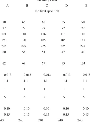
TABLE 5 Specifications for Automotive Gasoline (ASTM D 439-79)
Property Volatility Class
A B C D E
Octane number No limit specified
Distillation temperature, °C:
10% evaporated, max 70 65 60 55 50
50% evaporated, min 77 77 77 77 77
50% evaporated, max 121 118 116 113 110
90% evaporated, max 190 190 185 185 185
End point, max 225 225 225 225 225
Temperature for vapor-
liquid ratio of 20, min, °C 60 56 51 47 41
Vapor pressure, max, kPa
62 69 79 93 103
Lead content, max, g/L:
Unleaded grade 0.013 0.013 0.013 0.013 0.013
Conventional grade 1.1 1.1 1.1 1.1 1.1
Corrosion, copper strip, max, no.
1 1 1 1 1
Gum, existent, max, mg/100 mL
5 5 5 5 5
Sulfur, max, wt.%:
Unleaded grade 0.10 0.10 0.10 0.10 0.10
Conventional grade 0.15 0.15 0.15 0.15 0.15
Oxidation stability, min 240 240 240 240 240
< pr e viou s pa ge
page_9
n e x t pa ge >
Page 9For common gasoline engines the compression ratio is fixed. But the laboratory test engine has an adjustable head. Moving the head toward the piston increases the compression ratio and increases the tendency of a fuel to knock. To test a sample fuel, the compression ratio of the laboratory engine is set for track knockdetermined by a bouncing-pin
pressure gauge.
To relate the final engine conditions to an octane number, the knocking tendencies of two pure hydrocarbons are used as references. One of these hydrocarbons, isooctane (2,2,4-trimethyl pentane), is assigned an octane number of 100. The other, normal heptane, is assigned an octane number of zero. Mixtures of these reference hydrocarbons are assigned octane numbers equal to the volume percent of isooctane in the mixture. Then to complete the octane rating test, it is required to find the reference mixture that gives the same knock intensity in the test engine as that from the sample fuel. An exact match is not necessary, since the pressure gauge can be used to interpolate between near matches.
Research and Motor octane numbers identify other test engine variablesengine speed and intake air temperature. When
the engine runs at 600 r/min and with 125°F intake air temperature, the rating is called a Research octane number, abbreviated RON or simply R. When the engine is operated at 900 r/min and with 300°F intake air temperature, the rating is a Motor octane number, MON or M. Both ratings are important to a multicylinder automobile engine because it usually operates over a wide range of conditions. For marketing purposes, a compromise is used: the arithmetic average of the Research and Motor octane numbers, abbreviated (R+M)/2.
Leaded and unleaded grades denote whether the gasoline mix includes lead additives. Lead compounds such as
tetraethyl lead and tetramethyl lead are inexpensive additives to improve the octane rating of a gasoline mix. However, with the introduction of the catalytic muffler to automobile engines (to reduce exhaust emissions), unleaded gasolines were needed. Leaded fuel deactivated the catalyst in the muffler. The transition from an almost totally leaded gasoline market to an unleaded gasoline market is shown in Table 5.
Volatility is the third most popular marketing quality of a gasoline. Basically, volatility is a measure of a fuel's ability to
vaporize. It attempts to combine vapor pressures and boiling points for the many components of a gasoline blend. Volatility is related to the following engine performance parameters: easy starting, quick warm-up, freedom from carburetor icing, rapid acceleration, freedom from vapor lock, good manifold distribution, and minimum crankcase dilution.
In short, volatility compromises two extreme properties: enough low boiling hydrocarbons to vaporize easily in cold weather and enough high boiling hydrocarbons to remain a liquid in an engine's fuel supply system during hotter
periods. There must also be enough midboiling components to hold the mixture together. Several of the specifications in Table 5 relate to a fuel's volatility: distillation temperatures (used to determine volume percent vaporized for various conditions), temperature to achieve a 20 vaporliquid ratio, and Reid vapor pressure. The five volatility classes (A through E) are tied to seasonal temperatures and locations by a matrix (not shown here) based on typical weather conditions.
TABLE 6 Specifications for Aviation Gasolines (ASTM D 910-79)
10% evaporated, max 75 75 75
40% evaporated, min 75 75 75
50% evaporated, max 105 105 105
90% evaporated, max 135 135 135
Final boiling point, max 170 170 170
Vapor pressure, max, kPa
48 48 48
Net heat of combustion, min, kJ/kg 43,520 43,520 43,520 Corrosion, copper strip, max, no.
1 1 1
Gum, potential (5 h), max, mg/100 mL
6 6 6
Lead precipitate, visible, max, mg/100 mL
3 3 3
Aviation fuels are of two types: gasolines and jet fuels. The specifications for aviation gasolines are given in Table 6 and
Jet fuels are classified as "aviation turbine fuels," and their specifications are given in Table 7. In this case, ratings relative to octane number are replaced with properties concerned with the ability of the fuel to burn cleanly. These properties are discussed in the following section on diesel fuels.
DIESEL FUELS are distillates that are slightly heavier than gasoline. Diesel engines rely on compression-induced
ignition. This means diesel fuel must self-ignite easily. In other words, a diesel fuel needs a property that is the opposite of the antiknock property of gasoline. That opposite property is called cetane rating. The term is derived from the reference fuel, normal cetane, which is easily ignited by compression with air and is the basis for comparing diesel fuel blends. This and other specifications for diesel fuels are given in Table 8. Grade 1-D is a lighter material suitable for winter or low temperature operation. Grade 2-D is suitable for warmer temperature operation. Both of these grades have low sulfur content. Grade 4-D is for special situations where the fuel's flow properties and sulfur content are not critical.
TABLE 7 Specifications for Aviation Turbine Fuels (ASTM D 1655-80a)
Properties Jet A or A-1 Jet B
Density at 15°C,g/cm3 Viscosity at 20°C, max, mm2/s (= cSt)
8 Acidity, total, max, mg KOH/g
0.1 Net heat of combustion, min, kJ/kg
42,780 42,780
Corrosion, copper strip after 2 h at 100°C, max, n o. 1 1
Gum, existent, max, mg/100 mL
Sulfur has become one of the more important specifications for diesel fuels. The move is an attempt to further reduce sulfur in the
TABLE 8 Specifications for Diesel Fuel Oils (ASTM 97578)
Grade
Property 1-D 2-D 4-D
Distillation (90%) point, °C 288 max 282338
Flash point, min, °C
38 52 55
Water and sediment, max, vol.%
0.05 0.05 0.05
Carbon residue on 10% bottom, max, %
0.15 0.35
Ash, max, wt.%
0.01 0.01 0.01
Viscosity at 40°C, kinematic, mm2/s (= cSt)
1.32.4 1.94.1 5.524.0
Sulfur, max, wt.%
0.50 0.50 2.0
Corrosion, copper strip, max, no.
3 3
Cetane number, min
40 40 30
TABLE 9 Specifications for Fuel Oils (ASTM D 396-79)
max, vol.% 0.05 0.05 0.50 0.50 1.00 1.00 1.00 Carbon residue on
10% bottom, max, % 0.15 0.35
Ash, max, wt.% 0.10 0.10 0.10
Viscosity at 38°C, kinematic, mm2/s (= cSt):
min 1.4 2.0 2.0 5.8 26.4 65
The sulfur is chemically combined with the hydrocarbons. There are many possible combinations, but chemical analyses show sulfur compounds are in greater concentration in the heavier fractions of crude oil. When a sulfur-containing fuel is burned, the sulfur compounds are decomposed and the sulfur portion becomes sulfur oxides; usually sulfur dioxide and sulfur trioxide.
Typically, sulfur content is determined by burning a sample of the fuel in a specified apparatus. The combustion products are absorbed in a solution which can later be analyzed for sulfur, usually with a solution that forms barium sulfate. Results are reported as weight percent sulfur.
An indicative test for corrosive sulfur is the copper strip test. In this case a brightly polished copper strip is immersed in a fuel sample. During the test, any sulfur in the sample will tarnish the copper. The degree of tarnish is measured against three standards designated 1, 2, and 3; with the larger numbers representing a greater amount of corrosive sulfur.
FUEL OILS are also called heating oils and are distillates that cover a broad range of properties. For this reason, their specifications are not so
strict, as can be seen from the listing in Table 9. Some of their properties overlap specifications for the fuels mentioned earlier. Here are their grade definitions:
No. 1 fuel oilVery similar to kerosene or range oil (fuels used in stoves for cooking). This grade is defined as a distillate intended for vaporizing
in pot-type burners and other burners where a clean flame is required.
< pr e viou s pa ge
page_13
n e x t pa ge >
Page 13No. 2 fuel oilOften called domestic heating oil and having properties similar to diesel and heavier jet fuels. It is defined
as a distillate for general purpose heating in which the burners do not require the fuel to be completely vaporized before burning.
No. 4 fuel oilA light industrial heating oil. It is intended where preheating is not required for handling or burning. There
are two grades of No. 4 oil, differing primarily in safety (flash) and flow (viscosity) properties.
No. 5 fuel oilA heavy industrial oil. Preheating may be required for burning and, in cold climates, may be required for
handling.
No. 6 fuel oilA heavy residue oil sometimes called Bunker C when used to fuel ocean-going vessels. Preheating is
required for both handling and burning this grade oil.
NONFUEL PRODUCTS account for about 10% of the materials made from petroleum crude oil. These include
lubricants, waxes, asphalt, and petrochemical feedstocks. These topics are covered in this Encyclopedia in the
Lubricating Oil articles, Asphalt articles, Petrochemical articles, and Wax articles.
Petroleum Products, Production Costs Fabio Bernasconi
Production costs of refined petroleum products can be determined from a simple and accurate method that enables the user to calculate the break even value (BEV) to the refiner of all finished products from different grades of gasoline and middle distillate to specialties such as bitumens and lube basestocks.
The method, developed by the author, can also assess the effect on BEV of refinery configuration, mode of operation, and type of crude oil processes.
The BEV's are determined as a function of crude and residual fuel oil prices and are not influenced by the market price of the white products.
The ability to determine the production cost of a given product is a most valuable aid to the refiner, not just an academic exercise. Two important applications are ''make or buy" decisions to meet needs for incremental amounts of product above the refinery baseload and the possibility of focusing refining operation on products that show the highest contribution to overall margins.
For these reasons the determination of the production costs of petroleum products is a subject which is attracting
increasing interest. However, while it is relatively easy to calculate the overall cost of refining crude, it is not feasible to break this cost down by the various products produced. In fact, attempts to do so would be completely arbitrary.
On the other hand, by applying the incremental analysis technique to refining economics, it is possible to calculate the cost of producing an incremental amount of a specific product. In the refining industry this value is often assumed to be representative of the cost of production of that product, especially if in the calculation the "total" rather than the
"incremental" yields and variable costs for the various processing units are taken into account.
It should, however, be noted that even with this latter adjustment, the value calculated remains intrinsically the "incremental" and not the "total" cost of production. In other words, for a given refinery the weighted average of the calculated production costs for the various components of the production slate does not necessarily coincide with the total cost of refining crude oil though, in general, it is not too different from this value.
Methodology
The assessment of incremental production costs is generally done via linear programming (LP). The increasing availability of computer facilities has led to the construction of very large and sophisticated LP models that, if used properly, enable the refiner to achieve accurate results and analyze different operational situations with little effort. The drawback of these models is that the inexperienced or even the average user quickly loses control, as the model
complexity increases, of the factors which most influence the optimization process, and is, therefore, unable to interpret and criticize the results.
Misuse of the models in these circumstances can easily occur. Hence, frustration and distrust often accompany the use of these very powerful computer programs.
A way around this problem is to take advantage of simplified incremental analysis techniques (significantly more user friendly than the LP itself). They offer the advantage of clearly showing how the results are obtained. For general applications, the accuracy offered by these systems is quite satisfactory.
The methodology is based on a simplified version of the linear programming technique developed by the author, and is particularly suitable for analyzing refining operations. This methodology considers all the important factors that
determine the value of the various products to the refiner, but uses only a limited number of basic steps to arrive at the final result.
While maintaining a good overall accuracy, it offers the main advantage of an easy understanding. Another important feature of the methodology is its flexibility. It can be applied to calculate the production costs of both major products and specialties reflecting all conceivable refinery configurations and
< pr e viou s pa ge
page_15
n e x t pa ge >
Page 15mode of operations, and processing of any type of crude oil or alternative feedstock.
The methodology assesses the incremental variable cost of an oil product for a given refinery configuration by
analyzing the effect on overall operations of producing a marginal amount of that product above the refinery base load. It is assumed that in this process the production of the other white products should remain unchanged, which on an incremental basis is possible provided that the refinery runs on "balanced" operation.
The only two degrees of freedom left to the system are the crude oil requirement and the residual fuel oil production. It is therefore possible to obtain BEV formulas that express the incremental value of a product or stream as a function of the crude oil and residual fuel oil prices:
where P = product BEV, $/metric ton
C = crude oil cost, $/metric ton
F = residual fuel oil price, $/metric ton
V = incremental variable costs, $/metric ton of product
c = crude requirement (in weight) to produce one incremental ton of the product P
f = incremental residual fuel oil production (in weight) associated with production of one
incremental ton of the product P
The price of residual fuel oil, in turn, depends on its sulfur level, and it is therefore important to calculate, for each formula, the sulfur level of the incremental fuel oil produced. The value of this incremental fuel oil can be obtained by linear interpolation between the market price of a high- and a low-sulfur grade of fuel oil.
The BEV formulas also take into account the energy requirement for producing a given product which, reflecting actual operations, is subtracted directly from the total residual fuel oil production.
The energy requirement can be estimated from the BEV formulas by subtracting the product and fuel oil coefficients from the crude coefficient. The BEV formulas also show the incremental variable costs (primarily catalyst, chemicals, and power requirements) associated with the production of a given product.
The BEV formulas express the variable incremental cost of production only. Fixed costs such as labor, overheads, and depreciation, which cannot be quantified by incremental analysis, have to be added in order to assess the full production costs.
It is noteworthy that the BEV formulas are based entirely on a material balance. Hence, their validity is not affected by the actual crude oil price.
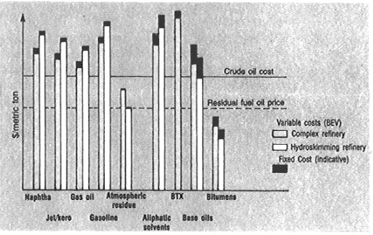
Figure 1 shows the relative production cost (BEV) of the major petroleum products and specialties calculated for two refinery configurations. In order to explain more in detail the principle on which the proposed methodology works, the BEV calculation for a few specific applications is discussed in the following examples.
< pr e viou s pa ge page_16 n e x t pa ge > Page 16
Fig. 1.
Relative BEV of major oil products and specialities.
White Distillate
The term "white distillate" is applied to all the refinery streams with a distillation range between approximately 80 and 360°C (at atmospheric pressure), and with properties similar to the corresponding straight-run distillate from atmospheric crude distillation. Light distillate products, i.e., naphthas, kerosene, jet fuels, diesel fuels, and heating oils, are all manufactured by appropriate blending of white distillate streams.
The value to the refiner of these products is therefore directly related to the value of the white distillate. The only difference is some additional hydrotreating cost, if required.
In a refinery the incremental value of the various white distillate streams suitable for blending into a finished light distillate product is, on a volume basis, the same. It is in fact possible, on an incremental basis, to shift naphtha into middle distillate, or vice versa, by adjusting the cut points of the crude distillation tower.
There is also no difference, as far as incremental value is concerned, between a straight run and a cracked stream, as long as both can be blended in the same finished product without exceeding a quality specification constraint.
The determination of the BEV of the white distillate pool in a refinery is the basic step for determining the value of any refined product. All the white products, besides the distillate products, are in fact produced by further processing of specific white distillate streams.
The cost evaluation of "black" products is also significantly affected by the white distillate value. These latter evaluations involve a comparison with the alternative of blending a heavy residue stream in the residual fuel oil pool,
the cost of which is dependent on the value of the cutter stock (a white distillate) required to make a marketable heavy fuel oil.
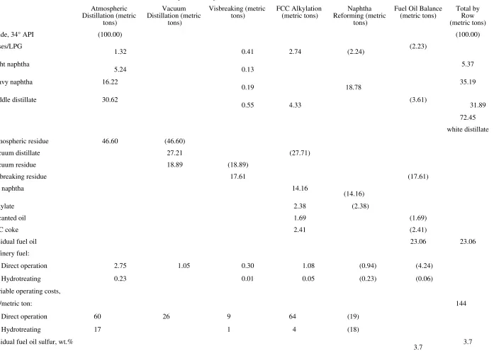
The data needed to derive the white distillate BEV formulas for two typical refinery configurations, i.e., hydroskimming and complex, are shown in Tables 1 and 2. In the complex configuration, vacuum distillation of the atmospheric residue is added to the hydroskimming base in order to recover a vacuum distillate stream which is then fed to a fluid catalytic cracker (FCC) with associated alkylation facilities. The vacuum residue undergoes a mild thermal upgrading in a visbreaker. In both cases the feedstock processed is a typical Middle East crude with gravity of 34°API.
The BEV calculation for the hydroskimming refinery is very simple, reflecting the simplicity of this configuration. It is based on two steps only. Crude is split into the relevant side streams in the crude atmospheric distillation tower, then a fuel oil balance is performed to calculate the amount of marketable residual fuel oil produced.
The total by row shows the incremental production of white distillate (light naphtha plus heavy naphtha plus middle distillate) and residual fuel oil obtainable by processing incrementally 100 tons of the given crude. It also shows the total variable operating cost involved with this operation.
The complex refinery case is conceptually more difficult. The atmospheric residue from distillation is sent to the
vacuum unit where the vacuum distillate cut is recovered from the residue and then fed to the upgrading facilitythe FCC plus alkylation block. The vacuum residue goes to the visbreaker.
TABLE 1 Incremental Formula Crude to White Distillate for Hydroskimming Refinery
Direct operation 60
Hydrotreating 17
Residual fuel oil sulfur, wt.% 2.4 2.4
Atmospheric
tons) FCC Alkylation (metric tons) Reforming (metric Naphtha tons)
Direct operation 2.75 1.05 0.30 1.08 (0.94) (4.24)
Hydrotreating 0.23 0.01 0.05 (0.23) (0.06)
Variable operating costs,
$/metric ton: 144
Direct operation 60 26 9 64 (19)
Hydrotreating 17 1 4 (18)
Residual fuel oil sulfur, wt.%
Among the upgraded streams, LCO and the thermally cracked light distillate can be assumed to be equivalent, on an incremental basis, to straight-run white distillate. However, this assumption is not valid for the cat naphtha and alkylate streams, which both have an intrinsically higher value than naphtha due to their relatively high octane characteristic. In a real operation, if incremental amounts of gasoline-blending stocks from upgrading facilities are released into the gasoline pool and the total gasoline production has to remain unchanged, the most logical refiner's action would be to back out some reformate from the pool. Following this logic, alkylate and cat naphtha are incrementally exchanged with an equivalent amount of reformate which is then run backward through the reformer to get straight-run naphtha.
The reforming yield in this step reflects a severity of operation to produce a reformate with the same octane quality as the blend of the cat naphtha and alkylate streams. Note than on an incremental basis, it is perfectly feasible to run a processing unit "backwards."
The last step is the fuel oil balance. It determines the amount of cutter stock required to produce a marketable fuel oil. This step also takes into account that a portion of the fuel oil pool has to be burned in the refinery to meet the processing units' energy requirements. The total by rows also shows that, for this configuration, it is possible to run incremental crude to produce only white distillate residual fuel oil.
The BEV formulas derived from the calculations for white distillate are shown by Table 3, which also summarizes the formulas for the other products considered.
TABLE 3 Examples of BEV Formulas White distillate:
Gasoline from incremental crude, 91 (R + M)/2:
Hydroskimming G = 2.2620C 1.1520F + 3.6
Complex G = 1.6148C 0.4848F + 4.8
Atmospheric residue:
Complex A = 0.6032C + 0.3959F 0.6
C = crude oil price in $/ton (34°API Middle East type)
F = residual fuel oil price in $/ton (the sulfur level for the hydroskimming and complex
cases is, respectively, 2.4 and 3.7 wt.%)
Fig. 2.
Comparison of gas oil BEV with spot price.
Naphtha and Gas Oil
The BEV's of naphtha and gas oil can be derived directly from the white distillate BEV formulas by taking into account the specific gravity effect. For naphtha, a further correction should be applied to reflect the volumetric crude expansion that follows the atmospheric distillation as a result of the nonideal behavior of the various hydrocarbons in the crude oil, and that occurs primarily in the naphtha and lighter fractions.
It is of interest to compare the calculated production costs with the spot market prices (Figs. 2 and 3). Note how closely in Fig. 2 the production cost of gas oil follows the spot price development, which confirms the accuracy of the BEV formulas.
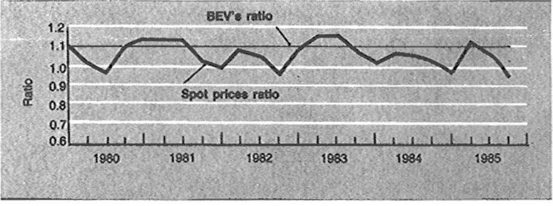
As expected, the complex refinery configuration enables the refiner to obtain production costs significantly lower than in the hydroskimming case. In the naphtha case, Fig. 3 compares the spot price ratio of naphtha and gas oil with the corresponding BEV ratio. The market price appears to be quite in line with production economics.
Fig. 3.
Naphtha to gas oil BEV's and spot prices.
< pr e viou s pa ge page_21 n e x t pa ge > Page 21
Gasoline
Gasoline production costs are very dependent on the manufacturing route and the quality specifications of the finished product. Typical production cases are:
Production from incremental crude, where gasoline is made by blending together all the suitable light streams, both straight run and cracked, produced by processing an incremental amount of crude. In this case the incremental gasoline blend reflects the average composition of the gasoline pool for the refinery configuration considered.
Production from naphtha reforming, where the incremental gasoline demand is met by reforming an incremental amount of straight run naphtha. This situation reflects primarily hydroskimming operations but, under particular circumstances, could apply also to conversion refineries.
< pr e viou s pa ge
page_22
n e x t pa ge >
Page 22The histrogram in Fig. 4 shows the difference in production costs resulting from the above three manufacturing cases for two gasoline grades, i.e., 81 and 91 (R+M)/2, which are generally representative of leaded premium (0.4 g/L), and the common grade of unleaded gasoline to be introduced in Western Europe.
The gasoline from naphtha (with naphtha produced from crude) and gasoline from incremental crude have very similar BEV's, with the former method showing some cost advantages. The difference increases with the octane level of the gasoline, reflecting the increasing operational difficulties in making gasoline from crude and in absorbing light naphtha and cat naphtha in the pool.
Addition of a light naphtha isomerization unit would greatly reduce this difference. The gasoline from the cracking operation appears to offer significantly lower production costs.
This benefit is due primarily to the advantage of starting from a relatively cheaper raw material, i.e., atmospheric residue as an alternative to crude, and not to an intrinsically cheaper processing route. The BEV of cracked gasoline is particularly sensitive to the pool octane quality, and increases sharply at high octane values due to the need for
reforming an increasing portion of the FCC gasoline prior to blending. Atmospheric Residue
The evaluation of atmospheric residue, also known as straight-run residual fuel oil, has attracted much interest since the early 1980s. This product has developed a large market as an upgrading feedstock alternative to crude oil. As a result, very little atmospheric residue is blended directly to residual fuel oil today. The evaluation of atmospheric residue, which is of interest primarily for upgrading refineries, is generally aimed at producing the following information: Determination of the amount of white distillate which can be obtained from the processing of the atmospheric residue. This approach implies that the atmospheric residue is equivalent to a heavy crude, as indeed it is in the case of a refinery equipped with residue upgrading facilities.
Determination of the BEV of the atmospheric residue as a function of crude and residual fuel oil values. This can be achieved by backing out from the refinery feedstock pool the amount of crude that would produce the same amount of white distillate as the atmospheric residue.
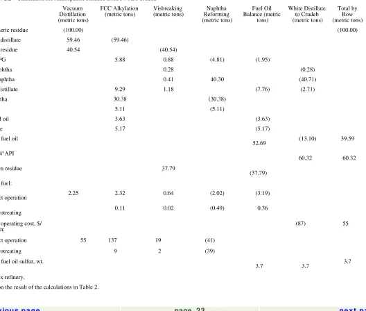
The BEV calculations are illustrated by Table 4. It is interesting to compare the developments of the spot price of high sulfur residual fuel oil with the calculated BEV of atmospheric residue (Fig. 5).
Vacuum Distillation (metric tons)
FCC Alkylation
(metric tons) Visbreaking (metric tons) Reforming Naphtha (metric tons)
Middle distillate 9.29 1.18 (7.76) (2.71)
Cat naphtha 30.38 (30.38)
Direct operation 2.25 2.32 0.64 (2.02) (3.19)
Hydrotreating 0.11 0.02 (0.49) 0.36
Variable operating cost, $/
metric ton: (87) 55
Direct operation 55 137 19 (41)
Hydrotreating 9 2 (39)
Residual fuel oil sulfur, wt.
% 3.7 3.7 3.7
aComplex refinery.
bBased on the result of the calculations in Table 2.
< pr e viou s pa ge page_24 n e x t pa ge > Page 24
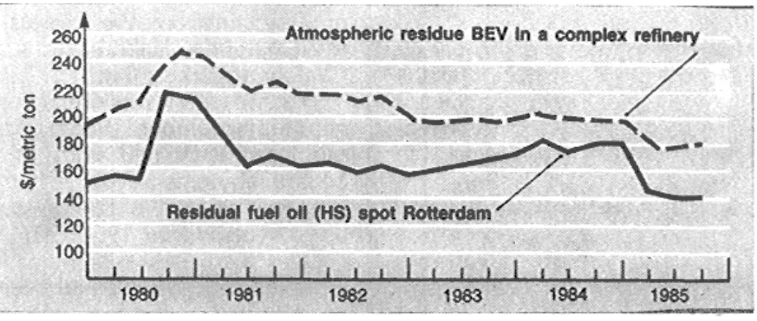
Fig. 5.
Atmospheric resid BEV and HSFO spot prices.
Considering that the premium commanded by this product over fuel oil fluctuated until the end of 1985 at around $15/ton, it is clear that processing this feedstock as an alternative to crude is an attractive proposition. It is also important to note how the differential between the atmospheric residue BEV and the spot residual fuel oil price narrowed during 1984 due to the unusually strong fuel oil price relative to the crude price.
The methodology has been tested extensively under different refining operating environments and has always provided reliable results. It should be noted that it does not replace linear programming, but simply complements it.
In fact, our methodology performs an economic analysis based on a given mode of operation without questioning whether this mode reflects the optimal way of processing crude. The optimization process is left to the LP and the refiner's experience.
In a sense, the methodology carries out a sensitivity analysis around the optimal LP solution. The advantage is that this task is achieved in a significantly more efficient and clear way than resorting to LP simulation.
The methodology is particularly suitable for implementation on a personal computer using available spreadsheet software. It has the potential to become a power tool for the refiner to support ''make or by" policies, planning decisions, and manufacturing-margins evaluations.
This material appeared in Oil & Gas Journal, pp. 2732, February 9, 1987, copyright © 1987 by Pennwell Publishing Co., Tulsa,
Oklahoma 74121, and is reprinted by special permission.
Octane Boosting John J. Lipinski Jack R. Wilcox
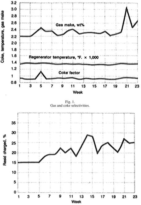
To meet additional octane requirements prompted by lead-phasedown rules, Coastal Eagle Point Oil Co. chose an octane-enhancing catalyst for its Westville, New Jersey, refinery. But octane enhancement was not the only benefit needed from the catalyst.
Coastal also had to increase the amount of resid charged to the fluid catalytic cracker (FCC) because of the nature of the crude oils processed in the refinery, and because of the operating nature of the crude and vacuum units. The
combination of octane enhancement and increased resid-charging capability was necessary to achieve acceptable economics for the overall operation.
The goal of improving gasoline octane while charging poor-quality feedstocks was achieved by switching to an ultrastable Y (USY) type catalyst, Filtrol ROC-1DY.
Background
Because of its key position in most refineries, the FCC unit must have the flexibility to process a wide variety of feeds. The operation of the cat cracker must also be adjusted and maintained at optimum conditions for maximum profitability. Some older cat crackers can be mechanically revamped to enable processing a wider range of feedstocks.
For example, upgrading regenerator and reactor internals, and the addition of heat-removal equipment, will allow for adding significant quantities of residual feeds to FCC combined feed. However, in many cases the use of the proper catalyst system, combined with appropriate unit operation, will also provide the refiner with a wider selection of feedstocks for the FCCU.
When faced with the economic reality of having to process heavier and poorer-quality feeds with a tighter capital budget, both refiners and catalyst manufacturers need to respond with innovative techniques to improve profitability. Generally, octane-improvement options are constrained by particular unit design and operating parameters. The most important parameters are:
Octane enhancing catalysts Operating severity
FCC gasoline end point Feedstock selection
< pr e viou s pa ge
page_26
n e x t pa ge >
Page 26The latter three criteria are routinely optimized by refineries in their quest to maintain profitability. Use of new catalysts may well be the remaining major step toward improving a given FCC's profitability without major capital expenditures. Ultrastable Zeolites
It had long been theorized that ultrastable Y zeolites (USY) could enhance both gasoline research and motor octane levels without a significant negative effect on gasoline selectivity. Using a series of laboratory-synthesized FCC catalysts, Pine et al. of Exxon demonstrated the effect of USY unit cell size on catalytic octane performance and activity. As the unit cell size of steam-deactivated, USY-containing catalysts decreased, there was a steady and
significant increase in both research and motor octane numbers, accompanied by a decreased microactivity test (MAT) activity and a strong tendency to make light C2 gas.
Also of considerable importance has been the USY's positive impact on coke selectivity.
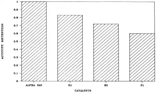
Filtrol's research concentrated on the development of a zeolite system, taking advantage of the attributes of the conventional USY while controlling the light gas production and maintaining acceptable activity levels. The result of this research effort was the development of dealuminated Y (DY) zeolite. Filtrol's dealuminated Y catalysts retain all the benefits of regular USY while maintaining better activity and producing less light gas. In addition, Filtrol combines USY technology with a cost-effective matrix in its catalysts for upgrading heavy gas oils and resids.
The effects of feed contaminants, particularly metals, has been well catalyst. These metals tend to nonselectively catalyze undesirable dehydrogenation reactions while also causing a loss of surface areas and zeolite activity. For units processing large quantities of resid containing high levels of nickel and vanadium, it is critical that a catalyst tolerate significant metals loading while continuing to provide good performance.
Coastal's Application
Coastal's Eagle Point refinery has improved FCC octanes without yield penalties while charging poor-quality feedstocks to the unit. This was accomplished primarily by switching to Filtrol ROC-1DY. This catalyst combines
octane-enhancing dealuminated zeolites with an active matrix to provide octane improvements together with the flexibility to process heavily contaminated poorer-quality feedstocks.