Getting Started with Python Data Analysis Learn to use powerful Python libraries for effective data processing and analysis pdf pdf

(1)

(2)

Getting Started with Python

Data Analysis

Learn to use powerful Python libraries for effective

data processing and analysis

Phuong Vo.T.H

(3)

[ FM-2 ]

Getting Started with Python Data Analysis

All rights reserved. No part of this book may be reproduced, stored in a retrieval system, or transmitted in any form or by any means, without the prior written permission of the publisher, except in the case of brief quotations embedded in critical articles or reviews.

Every effort has been made in the preparation of this book to ensure the accuracy of the information presented. However, the information contained in this book is sold without warranty, either express or implied. Neither the authors, nor Packt Publishing and its dealers and distributors will be held liable for any damages caused or alleged to be caused directly or indirectly by this book.

Packt Publishing has endeavored to provide trademark information about all of the companies and products mentioned in this book by the appropriate use of capitals. However, Packt Publishing cannot guarantee the accuracy of this information.

First published: October 2015

Production reference: 1231015

Published by Packt Publishing Ltd. Livery Place

35 Livery Street

Birmingham B3 2PB, UK.

ISBN 978-1-78528-511-0

(4)

Credits

Authors

Phuong Vo.T.H Martin Czygan

Reviewers

Dong Chao Hai Minh Nguyen Kenneth Emeka Odoh

Commissioning Editor

Dipika Gaonkar

Acquisition Editor

Harsha Bharwani

Content Development Editor

Shweta Pant

Technical Editor

Naveenkumar Jain

Copy Editors

Ting Baker Trishya Hajare

Project Coordinator

Sanjeet Rao

Proofreader Safis Editing

Indexer

Priya Sane

Production Coordinator

Nitesh Thakur

Cover Work

(5)

[ FM-4 ]

About the Authors

Phuong Vo.T.H

has a MSc degree in computer science, which is related to machine learning. After graduation, she continued to work in some companies as a data scientist. She has experience in analyzing users' behavior and building recommendation systems based on users' web histories. She loves to read machine learning and mathematics algorithm books, as well as data analysis articles.

(6)

About the Reviewers

Dong Chao

is both a machine learning hacker and a programmer. He’s currently conduct research on some Natural Language Processing field (sentiment analysis on sequences data) with deep learning in Tsinghua University. Before that he worked in XiaoMi one year ago, which is one of the biggest mobile communication companies in the world. He also likes functional programming and has some experience in Haskell and OCaml.

Hai Minh Nguyen

is currently a postdoctoral researcher at Rutgers University. He focuses on studying modified nucleic acid and designing Python interfaces for C++ and the Fortran library for Amber, a popular bimolecular simulation package. One of his notable achievements is the development of a pytraj program, a frontend of a C++ library that is designed to perform analysis of simulation data

(https://github.com/pytraj/pytraj).

Kenneth Emeka Odoh

presented a Python conference talk at Pycon, Finland, in 2012, where he spoke about Data Visualization in Django to a packed audience. He currently works as a graduate researcher at the University of Regina, Canada, in the field of visual analytics. He is a polyglot with experience in developing applications in C, C++, Python, and Java programming languages.

He has strong algorithmic and data mining skills. He is also a MOOC addict, as he spends time learning new courses about the latest technology.

(7)

[ FM-6 ]

www.PacktPub.com

Support files, eBooks, discount offers, and more

For support files and downloads related to your book, please visit

www.PacktPub.com.

Did you know that Packt offers eBook versions of every book published, with PDF and ePub files available? You can upgrade to the eBook version at www.PacktPub. com and as a print book customer, you are entitled to a discount on the eBook copy. Get in touch with us at service@packtpub.com for more details.

At www.PacktPub.com, you can also read a collection of free technical articles, sign up for a range of free newsletters and receive exclusive discounts and offers on Packt books and eBooks.

TM

https://www2.packtpub.com/books/subscription/packtlib

Do you need instant solutions to your IT questions? PacktLib is Packt's online digital book library. Here, you can search, access, and read Packt's entire library of books.

Why subscribe?

• Fully searchable across every book published by Packt • Copy and paste, print, and bookmark content

• On demand and accessible via a web browser

Free access for Packt account holders

(8)

Preface

The world generates data at an increasing pace. Consumers, sensors, or scientific experiments emit data points every day. In finance, business, administration and the natural or social sciences, working with data can make up a significant part of the job. Being able to efficiently work with small or large datasets has become a valuable skill.

There are a variety of applications to work with data, from spreadsheet applications, which are widely deployed and used, to more specialized statistical packages for experienced users, which often support domain-specific extensions for experts.

Python started as a general purpose language. It has been used in industry for a long time, but it has been popular among researchers as well. Around ten years ago, in 2006, the first version of NumPy was released, which made Python a first class language for numerical computing and laid the foundation for a prospering development, which led to what we today call the PyData ecosystem: A growing set of high-performance libraries to be used in the sciences, finance, business or anywhere else you want to work efficiently with datasets.

(13)

Preface

[ vi ]

And the outlook seems bright. Working with bigger datasets is getting simpler and sharing research findings and creating interactive programming notebooks has never been easier. It is the perfect moment to learn about data analysis in Python. This book lets you get started with a few core libraries of the PyData ecosystem: Numpy, Pandas, and matplotlib. In addition, two NoSQL databases are introduced. The final chapter will take a quick tour through one of the most popular machine learning libraries in Python.

We hope you find Python a valuable tool for your everyday data work and that we can give you enough material to get productive in the data analysis space quickly.

What this book covers

Chapter 1, Introducing Data Analysis and Libraries, describes the typical steps involved in a data analysis task. In addition, a couple of existing data analysis software packages are described.

Chapter 2, NumPy Arrays and Vectorized Computation, dives right into the core of the PyData ecosystem by introducing the NumPy package for high-performance computing. The basic data structure is a typed multidimensional array which supports various functions, among them typical linear algebra tasks. The data structure and functions are explained along with examples.

Chapter 3, Data Analysis with Pandas, introduces a prominent and popular data analysis library for Python called Pandas. It is built on NumPy, but makes a lot of real-world tasks simpler. Pandas comes with its own core data structures, which are explained in detail.

Chapter 4, Data Visualizaiton, focuses on another important aspect of data analysis: the understanding of data through graphical representations. The Matplotlib library is introduced in this chapter. It is one of the most popular 2D plotting libraries for Python and it is well integrated with Pandas as well.

Chapter 5, Time Series, shows how to work with time-oriented data in Pandas. Date and time handling can quickly become a difficult, error-prone task when implemented from scratch. We show how Pandas can be of great help there, by looking in detail at some of the functions for date parsing and date sequence generation.

Chapter 6, Interacting with Databases, deals with some typical scenarios. Your data

(14)

Preface

Chapter 7, Data Analysis Application Examples, applies many of the things covered in the previous chapters to deepen your understanding of typical data analysis workflows. How do you clean, inspect, reshape, merge, or group data – these are the concerns in this chapter. The library of choice in the chapter will be Pandas again.

Chapter 8, Machine Learning Models with scikit-learn, would like to make you familiar with a popular machine learning package for Python. While it supports dozens of models, we only look at four models, two supervised and two unsupervised. Even if this is not mentioned explicitly, this chapter brings together a lot of the existing tools. Pandas is often used for machine learning data preparation and matplotlib is used to create plots to facilitate understanding.

What you need for this book

There are not too many requirements to get started. You will need a Python programming environment installed on your system. Under Linux and Mac OS X, Python is usually installed by default. Installation on Windows is supported by an excellent installer provided and maintained by the community.

This book uses a recent Python 2, but many examples will work with Python 3 as well.

The versions of the libraries used in this book are the following: NumPy 1.9.2, Pandas 0.16.2, matplotlib 1.4.3, tables 3.2.2, pymongo 3.0.3, redis 2.10.3, and scikit-learn 0.16.1. As these packages are all hosted on PyPI, the Python package index, they can be easily installed with pip. To install NumPy, you would write:

$ pip install numpy

If you are not using them already, we suggest you take a look at virtual environments for managing isolating Python environment on your computer. For Python 2, there are two packages of interest there: virtualenv and

virtualenvwrapper. Since Python 3.3, there is a tool in the standard library called pyvenv (https://docs.python.org/3/library/venv.html), which serves the same purpose.

Most libraries will have an attribute for the version, so if you already have a library installed, you can quickly check its version:

(15)

Preface

[ viii ]

This works well for most libraries. A few, such as pymongo, use a different attribute (pymongo uses just version, without the underscores).

While all the examples can be run interactively in a Python shell, we recommend using IPython. IPython started as a more versatile Python shell, but has since

evolved into a powerful tool for exploration and sharing. We used IPython 4.0.0 with Python 2.7.10. IPython is a great way to work interactively with Python, be it in the terminal or in the browser.

Who this book is for

We assume you have been exposed to programming and Python and you want to broaden your horizons and get to know some key libraries in the data analysis field. We think that people with different backgrounds can benefit from this book. If you work in business, finance, in research and development at a lab or university, or if your work contains any data processing or analysis steps and you want know what Python has to offer, then this book can be of help. If you want to get started with basic data processing tasks or time series, then you can find lot of hands-on knowledge in the examples of this book. The strength of this book is its breadth. While we cannot dive very deep into a single package – although we will use Pandas extensively - we hope that we can convey a bigger picture: how the different parts of the Python data ecosystem work and can work together to form one of the most innovative and engaging programming environments.

Conventions

In this book, you will find a number of styles of text that distinguish between different kinds of information. Here are some examples of these styles, and an explanation of their meaning.

Code words in text, database table names, folder names, filenames, file extensions, pathnames, dummy URLs, user input, and Twitter handles are shown as follows: "We can include other contexts through the use of the include directive."

A block of code is set as follows:

>>> import numpy as np >>> np.random.randn()

When we wish to draw your attention to a particular part of a code block, the relevant lines or items are set in bold:

(16)

Preface

Any command-line input or output is written as follows:

$ cat "data analysis" | wc -l

New terms and important words are shown in bold. Words that you see on the screen, in menus or dialog boxes for example, appear in the text like this: "clicking the Next button moves you to the next screen".

Warnings or important notes appear in a box like this.

Tips and tricks appear like this.

Reader feedback

Feedback from our readers is always welcome. Let us know what you think about this book—what you liked or may have disliked. Reader feedback is important for us to develop titles that you really get the most out of.

To send us general feedback, simply send an e-mail to feedback@packtpub.com, and mention the book title via the subject of your message.

If there is a topic that you have expertise in and you are interested in either writing or contributing to a book, see our author guide on www.packtpub.com/authors.

Customer support

Now that you are the proud owner of a Packt book, we have a number of things to help you to get the most from your purchase.

Downloading the example code

(17)

Preface

[ x ]

Errata

Although we have taken every care to ensure the accuracy of our content, mistakes do happen. If you find a mistake in one of our books—maybe a mistake in the text or the code—we would be grateful if you would report this to us. By doing so, you can save other readers from frustration and help us improve subsequent versions of this book. If you find any errata, please report them by visiting http://www.packtpub. com/submit-errata, selecting your book, clicking on the erratasubmissionform link, and entering the details of your errata. Once your errata are verified, your submission will be accepted and the errata will be uploaded on our website, or added to any list of existing errata, under the Errata section of that title. Any existing errata can be viewed by selecting your title from http://www.packtpub.com/support.

Piracy

Piracy of copyright material on the Internet is an ongoing problem across all media. At Packt, we take the protection of our copyright and licenses very seriously. If you come across any illegal copies of our works, in any form, on the Internet, please provide us with the location address or website name immediately so that we can pursue a remedy.

Please contact us at copyright@packtpub.com with a link to the suspected pirated material.

We appreciate your help in protecting our authors, and our ability to bring you valuable content.

Questions

(18)

Introducing Data Analysis

and Libraries

Data is raw information that can exist in any form, usable or not. We can easily get data everywhere in our lives; for example, the price of gold on the day of writing was $ 1.158 per ounce. This does not have any meaning, except describing the price of gold. This also shows that data is useful based on context.

With the relational data connection, information appears and allows us to expand our knowledge beyond the range of our senses. When we possess gold price data gathered over time, one piece of information we might have is that the price has continuously risen from $1.152 to $1.158 over three days. This could be used by someone who tracks gold prices.

(19)

Introducing Data Analysis and Libraries

[ 2 ]

The following figure illustrates the steps from data to knowledge; we call this process, the data analysis process and we will introduce it in the next section:

Data Collecting Summarizing

organizing

Gold price today is 1158$

Gold price has risen for three days

Gold price will slightly decrease on next day Knowledge

Information

Decision making Synthesising

Analysing

In this chapter, we will cover the following topics:

• Data analysis and process

• An overview of libraries in data analysis using different programming languages

• Common Python data analysis libraries

Data analysis and processing

Data is getting bigger and more diverse every day. Therefore, analyzing and processing data to advance human knowledge or to create value is a big challenge. To tackle these challenges, you will need domain knowledge and a variety of skills, drawing from areas such as computer science, artificial intelligence (AI) and

(20)

Chapter 1

Computer Science

Artificial Intelligent & Machine Learning

Knowledge Domain

Statistics & Mathematics Data Analysis

Math_....

Data expertise ....

Algorithms ....

Programming....

Let's go through data analysis and its domain knowledge:

• Computer science: We need this knowledge to provide abstractions for efficient data processing. Basic Python programming experience is required to follow the next chapters. We will introduce Python libraries used in data analysis.

• Artificial intelligence and machine learning: If computer science knowledge helps us to program data analysis tools, artificial intelligence and machine learning help us to model the data and learn from it in order to build smart products.

• Statistics and mathematics: We cannot extract useful information from raw data if we do not use statistical techniques or mathematical functions. • Knowledge domain: Besides technology and general techniques, it is

(21)

[ 4 ]

Data analysis is a process composed of the following steps:

• Data requirements: We have to define what kind of data will be collected based on the requirements or problem analysis. For example, if we want to detect a user's behavior while reading news on the internet, we should be aware of visited article links, dates and times, article categories, and the time the user spends on different pages.

• Data collection: Data can be collected from a variety of sources: mobile, personal computer, camera, or recording devices. It may also be obtained in different ways: communication, events, and interactions between person and person, person and device, or device and device. Data appears whenever and wherever in the world. The problem is how we can find and gather it to solve our problem? This is the mission of this step.

• Data processing: Data that is initially obtained must be processed or organized for analysis. This process is performance-sensitive. How fast can we create, insert, update, or query data? When building a real product that has to process big data, we should consider this step carefully. What kind of database should we use to store data? What kind of data structure, such as analysis, statistics, or visualization, is suitable for our purposes?

• Data cleaning: After being processed and organized, the data may still contain duplicates or errors. Therefore, we need a cleaning step to reduce those situations and increase the quality of the results in the following steps. Common tasks include record matching, deduplication, and column segmentation. Depending on the type of data, we can apply several types of data cleaning. For example, a user's history of visits to a news website might contain a lot of duplicate rows, because the user might have refreshed certain pages many times. For our specific issue, these rows might not carry any meaning when we explore the user's behavior so we should remove them before saving it to our database. Another situation we may encounter is click fraud on news—someone just wants to improve their website ranking or sabotage awebsite. In this case, the data will not help us to explore a user's behavior. We can use thresholds to check whether a visit page event comes from a real person or from malicious software.

(22)

Chapter 1

• Modelling and algorithms: A lot of mathematical formulas and algorithms may be applied to detect or predict useful knowledge from the raw data. For example, we can use similarity measures to cluster users who have exhibited similar news-reading behavior and recommend articles of interest to them next time. Alternatively, we can detect users' genders based on their news reading behavior by applying classification models such as the Support

Vector Machine (SVM) or linear regression. Depending on the problem, we may use different algorithms to get an acceptable result. It can take a lot of time to evaluate the accuracy of the algorithms and choose the best one to implement for a certain product.

• Data product: The goal of this step is to build data products that receive data input and generate output according to the problem requirements. We will apply computer science knowledge to implement our selected algorithms as well as manage the data storage.

An overview of the libraries in data

analysis

There are numerous data analysis libraries that help us to process and analyze data. They use different programming languages, and have different advantages and disadvantages of solving various data analysis problems. Now, we will introduce some common libraries that may be useful for you. They should give you an overview of the libraries in the field. However, the rest of this book focuses on Python-based libraries.

Some of the libraries that use the Java language for data analysis are as follows:

(23)

[ 6 ]

• Mallet: This is another Java library that is used for statistical natural language processing, document classification, clustering, topic modeling, information extraction, and other machine-learning applications on text. There is an add-on package for Mallet, called GRMM, that contains support for inference in general, graphical models, and training of Conditional

random fields (CRF) with arbitrary graphical structures. In my experience, the library performance and the algorithms are better than Weka. However, its only focus is on text-processing problems. The reference page is at http://mallet.cs.umass.edu/.

• Mahout: This is Apache's machine-learning framework built on top of Hadoop; its goal is to build a scalable machine-learning library. It looks promising, but comes with all the baggage and overheads of Hadoop. The homepage is at http://mahout.apache.org/.

• Spark: This is a relatively new Apache project, supposedly up to a hundred times faster than Hadoop. It is also a scalable library that consists of common machine-learning algorithms and utilities. Development can be done in Python as well as in any JVM language. The reference page is at https://spark.apache.org/docs/1.5.0/mllib-guide.html.

Here are a few libraries that are implemented in C++:

• Vowpal Wabbit: This library is a fast, out-of-core learning system sponsored by Microsoft Research and, previously, Yahoo! Research. It has been

used to learn a tera-feature (1012) dataset on 1,000 nodes in one hour. More information can be found in the publication at http://arxiv.org/ abs/1110.4198.

• MultiBoost: This package is a multiclass, multi label, and multitask classification boosting software implemented in C++. If you use this software, you should refer to the paper published in 2012 in the JournalMachine Learning Research, MultiBoost: A Multi-purpose Boosting Package, D.Benbouzid, R. Busa-Fekete, N. Casagrande, F.-D. Collin, and B. Kégl. • MLpack: This is also a C++ machine-learning library, developed by the

Fundamental Algorithmic and Statistical Tools Laboratory (FASTLab) at Georgia Tech. It focusses on scalability, speed, and ease-of-use, and was presented at the BigLearning workshop of NIPS 2011. Its homepage is at http://www.mlpack.org/about.html.

(24)

Chapter 1

Other libraries for data processing and analysis are as follows:

• Statsmodels: This is a great Python library for statistical modeling and is mainly used for predictive and exploratory analysis.

• Modular toolkit for data processing (MDP): This is a collection of

supervised and unsupervised learning algorithms and other data processing units that can be combined into data processing sequences and more complex feed-forward network architectures (http://mdp-toolkit.sourceforge. net/index.html).

• Orange: This is an open source data visualization and analysis for novices and experts. It is packed with features for data analysis and has add-ons for bioinformatics and text mining. It contains an implementation of self-organizing maps, which sets it apart from the other projects as well (http://orange.biolab.si/).

• Mirador: This is a tool for the visual exploration of complex datasets,

supporting Mac and Windows. It enables users to discover correlation patterns and derive new hypotheses from data (http://orange.biolab.si/).

• RapidMiner: This is another GUI-based tool for data mining, machine learning, and predictive analysis (https://rapidminer.com/).

• Theano: This bridges the gap between Python and lower-level languages. Theano gives very significant performance gains, particularly for large matrix operations, and is, therefore, a good choice for deep learning models. However, it is not easy to debug because of the additional compilation layer. • Natural language processing toolkit (NLTK): This is written in Python with

very unique and salient features.

Here, I could not list all libraries for data analysis. However, I think the above libraries are enough to take a lot of your time to learn and build data analysis applications. I hope you will enjoy them after reading this book.

Python libraries in data analysis

(25)

[ 8 ]

NumPy

One of the fundamental packages used for scientific computing in Python is Numpy. Among other things, it contains the following:

• A powerful N-dimensional array object

• Sophisticated (broadcasting) functions for performing array computations • Tools for integrating C/C++ and Fortran code

• Useful linear algebra operations, Fourier transformations, and random number capabilities

Besides this, it can also be used as an efficient multidimensional container of generic data. Arbitrary data types can be defined and integrated with a wide variety of databases.

Pandas

Pandas is a Python package that supports rich data structures and functions for analyzing data, and is developed by the PyData Development Team. It is focused on the improvement of Python's data libraries. Pandas consists of the following things:

• A set of labeled array data structures; the primary of which are Series, DataFrame, and Panel

• Index objects enabling both simple axis indexing and multilevel/hierarchical axis indexing

• An intergraded group by engine for aggregating and transforming datasets • Date range generation and custom date offsets

• Input/output tools that load and save data from flat files or PyTables/HDF5 format

• Optimal memory versions of the standard data structures

• Moving window statistics and static and moving window linear/panel regression

(26)

Chapter 1

Matplotlib

Matplotlib is the single most used Python package for 2D-graphics. It provides both a very quick way to visualize data from Python and publication-quality figures in many formats: line plots, contour plots, scatter plots, and Basemap plots. It comes with a set of default settings, but allows customization of all kinds of properties. However, we can easily create our chart with the defaults of almost every property in Matplotlib.

PyMongo

MongoDB is a type of NoSQL database. It is highly scalable, robust, and perfect to work with JavaScript-based web applications, because we can store data as JSON documents and use flexible schemas.

PyMongo is a Python distribution containing tools for working with MongoDB. Many tools have also been written for working with PyMongo to add more features such as MongoKit, Humongolus, MongoAlchemy, and Ming.

The scikit-learn library

The scikit-learn is an open source machine-learning library using the Python programming language. It supports various machine learning models, such as classification, regression, and clustering algorithms, interoperated with the Python numerical and scientific libraries NumPy and SciPy. The latest scikit-learn version is 0.16.1, published in April 2015.

Summary

In this chapter, we presented three main points. Firstly, we figured out the

(27)

[ 10 ]

Practice exercise

The following table describes users' rankings on Snow White movies:

UserID Sex Location Ranking

A Male Philips 4

B Male VN 2

C Male Canada 1 D Male Canada 2

E Female VN 5

F Female NY 4

Exercise 1: What information can we find in this table? What kind of knowledge can we derive from it?

(28)

NumPy Arrays and

Vectorized Computation

NumPy is the fundamental package supported for presenting and computing data with high performance in Python. It provides some interesting features as follows:

• Extension package to Python for multidimensional arrays (ndarrays), various derived objects (such as masked arrays), matrices providing vectorization operations, and broadcasting capabilities. Vectorization can significantly increase the performance of array computations by taking advantage of Single Instruction Multiple Data (SIMD) instruction sets in modern CPUs.

• Fast and convenient operations on arrays of data, including mathematical manipulation, basic statistical operations, sorting, selecting, linear algebra, random number generation, discrete Fourier transforms, and so on.

• Efficiency tools that are closer to hardware because of integrating C/C++/Fortran code.

(29)

NumPy Arrays and Vectorized Computation

[ 12 ]

NumPy arrays

An array can be used to contain values of a data object in an experiment or

simulation step, pixels of an image, or a signal recorded by a measurement device. For example, the latitude of the Eiffel Tower, Paris is 48.858598 and the longitude is 2.294495. It can be presented in a NumPy array object as p:

>>> import numpy as np

>>> p = np.array([48.858598, 2.294495]) >>> p

Output: array([48.858598, 2.294495])

This is a manual construction of an array using the np.array function. The standard convention to import NumPy is as follows:

>>> import numpy as np

You can, of course, put from numpy import * in your code to avoid having to write np. However, you should be careful with this habit because of the potential code conflicts (further information on code conventions can be found in the Python Style Guide, also known as PEP8, at https://www.python.org/dev/peps/pep-0008/). There are two requirements of a NumPy array: a fixed size at creation and a uniform, fixed data type, with a fixed size in memory. The following functions help you to get information on the p matrix:

>>> p.ndim # getting dimension of array p 1

>>> p.shape # getting size of each array dimension (2,)

>>> len(p) # getting dimension length of array p 2

>>> p.dtype # getting data type of array p dtype('float64')

Data types

(30)

Chapter 2

See the following table for a listing of NumPy's supported data types:

Type Type

code Description Range of value bool Boolean stored as a byte True/False

intc _{Similar to C int (int32 or int}

64)

intp Integer used for indexing

(same as C size_t)

int8, uint8 i1, u1 Signed and unsigned 8-bit integer types

int8: (-128 to 127) uint8: (0 to 255)

int16,

uint16

i2, u2 Signed and unsigned 16-bit integer types

int16: (-32768 to 32767) uint16: (0 to 65535)

int32,

uint32

I4, u4 Signed and unsigned 32-bit integer types

i8, u8 Signed and unsigned 64-bit integer types

Int64: (-9223372036854775808

to 9223372036854775807)

uint64: (0 to

18446744073709551615)

float16 _f2 _{Half precision float: sign bit,}

5 bits exponent, and 10b bits mantissa

float32 f4 / f Single precision float: sign bit, 8 bits exponent, and 23 bits mantissa

float64 _{f8 / d} _{Double precision float: sign}

bit, 11 bits exponent, and 52 bits mantissa represented by two 32-bit, 64-bit, and 128-bit floats

object 0 Python object type

string_ _S _{Fixed-length string type} _{Declare a string}dtype with length 10, using S10

unicode_ _U _{Fixed-length Unicode type} _{Similar to string_ example, we}

(31)

[ 14 ]

We can easily convert or cast an array from one dtype to another using the astype method:

The astype function will create a new array with a copy of data from an old array, even though the new dtype is similar to the old one.

Array creation

There are various functions provided to create an array object. They are very useful for us to create and store data in a multidimensional array in different situations.

Now, in the following table we will summarize some of NumPy's common functions and their use by examples for array creation:

Function Description Example empty,

empty_like

Create a new array of the given shape and type, without ones on the diagonal and zero elsewhere

>>> np.eye(2, dtype=np.int) array([[1, 0], [0, 1]])

ones, ones_ like

Create a new array with the given shape and type, filled with 1s for all elements

>>> np.ones(5)

array([1., 1., 1., 1., 1.]) >>> np.ones(4, dtype=np.int) array([1, 1, 1, 1])

>>> x = np.array([[0,1,2], [3,4,5]]) >>> np.ones_like(x)

(32)

Chapter 2

Function Description Example zeros,

zeros_like

This is similar to

ones, ones_like,

arange Create an array with even spaced values

Create a new array with the given shape and type, filled with a selected value

array _{Create an array from}

the existing data

>>> np.array([[1.1, 2.2, 3.3], [4.4, 5.5, 6.6]])

array([1.1, 2.2, 3.3], [4.4, 5.5, 6.6]])

asarray Convert the input to an array

>>> a = [3.14, 2.46] >>> np.asarray(a) array([3.14, 2.46])

copy Return an array copy of the given object

>>> a = np.array([[1, 2], [3, 4]]) >>> np.copy(a)

array([[1, 2], [3, 4]])

fromstring Create 1-D array from a string or text

>>> np.fromstring('3.14 2.17', dtype=np.float, sep=' ')

(33)

[ 16 ]

Indexing and slicing

As with other Python sequence types, such as lists, it is very easy to access and assign a value of each array's element:

>>> a = np.arange(7) >>> a

array([0, 1, 2, 3, 4, 5, 6]) >>> a[1], a [4], a[-1] (1, 4, 6)

In Python, array indices start at 0. This is in contrast to Fortran or Matlab, where indices begin at 1.

As another example, if our array is multidimensional, we need tuples of integers to index an item:

>>> a = np.array([[1, 2, 3], [4, 5, 6], [7, 8, 9]]) >>> a[0, 2] # first row, third column

3

>>> a[0, 2] = 10 >>> a

array([[1, 2, 10], [4, 5, 6], [7, 8, 9]]) >>> b = a[2]

>>> b

array([7, 8, 9]) >>> c = a[:2] >>> c

array([[1, 2, 10], [4, 5, 6]])

We call b and c as array slices, which are views on the original one. It means that the data is not copied to b or c, and whenever we modify their values, it will be reflected in the array a as well:

>>> b[-1] = 11 >>> a

array([[1, 2, 10], [4, 5, 6], [7, 8, 11]])

(34)

Chapter 2

Fancy indexing

Besides indexing with slices, NumPy also supports indexing with Boolean or integer arrays (masks). This method is called fancy indexing. It creates copies, not views.

First, we take a look at an example of indexing with a Boolean mask array:

>>> a = np.array([3, 5, 1, 10]) >>> b = (a % 5 == 0)

>>> b

array([False, True, False, True], dtype=bool) >>> c = np.array([[0, 1], [2, 3], [4, 5], [6, 7]]) >>> c[b]

array([[2, 3], [6, 7]])

The second example is an illustration of using integer masks on arrays:

>>> a = np.array([[1, 2, 3, 4], [5, 6, 7, 8],

[9, 10, 11, 12], [13, 14, 15, 16]]) >>> a[[2, 1]]

array([[9, 10, 11, 12], [5, 6, 7, 8]])

>>> a[[-2, -1]] # select rows from the end array([[ 9, 10, 11, 12], [13, 14, 15, 16]])

>>> a[[2, 3], [0, 1]] # take elements at (2, 0) and (3, 1) array([9, 14])

The mask array must have the same length as the axis that it's indexing.

Downloading the example code

You can download the example code files for all Packt books

you have purchased from your account at http://www. packtpub.com. If you purchased this book elsewhere, you can visit http://www.packtpub.com/support and register to

(35)

[ 18 ]

Numerical operations on arrays

We are getting familiar with creating and accessing ndarrays. Now, we continue to the next step, applying some mathematical operations to array data without writing any for loops, of course, with higher performance.

Scalar operations will propagate the value to each element of the array:

>>> a = np.ones(4) >>> a * 2

array([2., 2., 2., 2.]) >>> a + 3

array([4., 4., 4., 4.])

All arithmetic operations between arrays apply the operation element wise:

>>> a = np.ones([2, 4]) >>> a * a

array([[1., 1., 1., 1.], [1., 1., 1., 1.]]) >>> a + a

array([[2., 2., 2., 2.], [2., 2., 2., 2.]])

Also, here are some examples of comparisons and logical operations:

>>> a = np.array([1, 2, 3, 4]) >>> b = np.array([1, 1, 5, 3]) >>> a == b

array([True, False, False, False], dtype=bool)

>>> np.array_equal(a, b) # array-wise comparison False

>>> c = np.array([1, 0]) >>> d = np.array([1, 1])

(36)

Chapter 2

Array functions

Many helpful array functions are supported in NumPy for analyzing data. We will list some part of them that are common in use. Firstly, the transposing function is another kind of reshaping form that returns a view on the original data array without copying anything:

>>> a = np.array([[0, 5, 10], [20, 25, 30]]) >>> a.reshape(3, 2)

array([[0, 5], [10, 20], [25, 30]]) >>> a.T

array([[0, 20], [5, 25], [10, 30]])

In general, we have the swapaxes method that takes a pair of axis numbers and returns a view on the data, without making a copy:

>>> a = np.array([[[0, 1, 2], [3, 4, 5]], [[6, 7, 8], [9, 10, 11]]])

>>> a.swapaxes(1, 2) array([[[0, 3], [1, 4], [2, 5]], [[6, 9], [7, 10], [8, 11]]])

The transposing function is used to do matrix computations; for example, computing the inner matrix product XT.X using np.dot:

>>> a = np.array([[1, 2, 3],[4,5,6]]) >>> np.dot(a.T, a)

(37)

[ 20 ]

Sorting data in an array is also an important demand in processing data. Let's take a look at some sorting functions and their use:

>>> a = np.array ([[6, 34, 1, 6], [0, 5, 2, -1]])

>>> np.sort(a) # sort along the last axis array([[1, 6, 6, 34], [-1, 0, 2, 5]])

>>> np.sort(a, axis=0) # sort along the first axis array([[0, 5, 1, -1], [6, 34, 2, 6]])

>>> b = np.argsort(a) # fancy indexing of sorted array >>> b

array([[2, 0, 3, 1], [3, 0, 2, 1]]) >>> a[0][b[0]]

array([1, 6, 6, 34])

>>> np.argmax(a) # get index of maximum element 1

See the following table for a listing of array functions:

Function Description Example

>>> a = np.array([0.,30., 45.]) >>> np.sin(a * np.pi / 180) array([0., 0.5, 0.7071678])

(38)

Chapter 2

With the NumPy package, we can easily solve many kinds of data processing tasks without writing complex loops. It is very helpful for us to control our code as well as the performance of the program. In this part, we want to introduce some mathematical and statistical functions.

See the following table for a listing of mathematical and statistical functions:

Function Description Example sum _{Calculate the sum}

of all the elements in an array or along the axis

>>> a = np.array([[2,4], [3,5]]) >>> np.sum(a, axis=0)

cross _{Return the cross}

product of two arrays

(39)

>>> np.where([[True, True], [False, True]], [[1,2],[3,4]], [[5,6],[7,8]]) array([[1,2], [7, 4]])

unique Return the sorted unique values in

>>> b = np.array(['a', 'xyz', 'klm', 'd'])

>>> np.intersect1d(a,b)

array(['a', 'd'], dtype='|S3')

Loading and saving data

We can also save and load data to and from a disk, either in text or binary format, by using different supported functions in NumPy package.

Saving an array

Arrays are saved by default in an uncompressed raw binary format, with the file extension .npy by the np.save function:

(40)

Chapter 2

The library automatically assigns the .npy extension, if we omit it.

If we want to store several arrays into a single file in an uncompressed .npz format, we can use the np.savez function, as shown in the following example:

>>> a = np.arange(4) >>> b = np.arange(7)

>>> np.savez('test2.npz', arr0=a, arr1=b)

The .npz file is a zipped archive of files named after the variables they contain. When we load an .npz file, we get back a dictionary-like object that can be queried for its lists of arrays:

>>> dic = np.load('test2.npz') >>> dic['arr0']

array([0, 1, 2, 3])

Another way to save array data into a file is using the np.savetxt function that allows us to set format properties in the output file:

>>> x = np.arange(4)

>>> # e.g., set comma as separator between elements >>> np.savetxt('test3.out', x, delimiter=',')

Loading an array

We have two common functions such as np.load and np.loadtxt, which correspond to the saving functions, for loading an array:

>>> np.load('test1.npy') array([[0, 1, 2], [3, 4, 5]])

>>> np.loadtxt('test3.out', delimiter=',') array([0., 1., 2., 3.])

(41)

[ 24 ]

Linear algebra with NumPy

Linear algebra is a branch of mathematics concerned with vector spaces and the mappings between those spaces. NumPy has a package called linalg that supports powerful linear algebra functions. We can use these functions to find eigenvalues and eigenvectors or to perform singular value decomposition:

>>> A = np.array([[1, 4, 6], [5, 2, 2],

[-1, 6, 8]])

>>> w, v = np.linalg.eig(A)

>>> w # eigenvalues

array([-0.111 + 1.5756j, -0.111 – 1.5756j, 11.222+0.j]) >>> v # eigenvector

array([[-0.0981 + 0.2726j, -0.0981 – 0.2726j, 0.5764+0.j], [0.7683+0.j, 0.7683-0.j, 0.4591+0.j],

[-0.5656 – 0.0762j, -0.5656 + 0.00763j, 0.6759+0.j]])

The function is implemented using the geev Lapack routines that compute the eigenvalues and eigenvectors of general square matrices.

Another common problem is solving linear systems such as Ax = b with A as a matrix and x and b as vectors. The problem can be solved easily using the numpy.linalg.solve function:

>>> A = np.array([[1, 4, 6], [5, 2, 2], [-1, 6, 8]]) >>> b = np.array([[1], [2], [3]])

>>> x = np.linalg.solve(A, b) >>> x

array([[-1.77635e-16], [2.5], [-1.5]])

The following table will summarise some commonly used functions in the numpy. linalg package:

Function Description Example dot _{Calculate the dot}

product of two arrays

>>> a = np.array([[1, 0],[0, 1]]) >>> b = np.array( [[4, 1],[2, 2]]) >>> np.dot(a,b)

(42)

Chapter 2

Function Description Example inner, outer Calculate the inner and

outer product of two arrays

>>> a = np.array([1, 1, 1]) >>> b = np.array([3, 5, 1]) >>> np.inner(a,b)

9

linalg.norm _{Find a matrix or vector}

norm

linalg.inv _{Compute the inverse of}

a matrix

>>> a = np.array([[1,2],[3,4]]) >>> np.linalg.inv(a)

array([[-2., 1.],[1.5, -0.5]])

linalg.qr Calculate the QR decomposition

>>> a = np.array([[1,2],[3,4]]) >>> np.linalg.qr(a)

(array([[0.316, 0.948], [0.948, 0.316]]), array([[ 3.162, 4.427], [ 0., 0.632]]))

linalg.cond _{Compute the condition}

number of a matrix

>>> a = np.array([[1,3],[2,4]]) >>> np.linalg.cond(a)

14.933034

trace _{Compute the sum of the}

diagonal element

>>> np.trace(np.arange(6)). reshape(2,3))

4

NumPy random numbers

An important part of any simulation is the ability to generate random numbers. For this purpose, NumPy provides various routines in the submodule random. It uses a particular algorithm, called the Mersenne Twister, to generate

(43)

[ 26 ]

First, we need to define a seed that makes the random numbers predictable. When the value is reset, the same numbers will appear every time. If we do not assign the seed, NumPy automatically selects a random seed value based on the system's random number generator device or on the clock:

>>> np.random.seed(20)

An array of random numbers in the [0.0, 1.0] interval can be generated as follows:

>>> np.random.rand(5)

array([0.5881308, 0.89771373, 0.89153073, 0.81583748, 0.03588959])

>>> np.random.rand(5)

array([0.69175758, 0.37868094, 0.51851095, 0.65795147, 0.19385022])

>>> np.random.seed(20) # reset seed number >>> np.random.rand(5)

array([0.5881308, 0.89771373, 0.89153073, 0.81583748, 0.03588959])

If we want to generate random integers in the half-open interval [min, max], we can user the randint(min, max, length) function:

>>> np.random.randint(10, 20, 5) array([17, 12, 10, 16, 18])

NumPy also provides for many other distributions, including the Beta,

(44)

Chapter 2

The following table will list some distribution functions and give examples for generating random numbers:

Function Description Example binomial Draw samples from a

binomial distribution

dirichlet _{Draw samples using a}

Dirichlet distribution

poisson Draw samples from a Poisson distribution

>>> np.random.poisson(lam=2, size= 2)

array([4,1])

normal Draw samples using a normal Gaussian distribution

>>> np.random.normal

(loc=2.5, scale=0.3, size=3) array([2.4436, 2.849, 2.741)

uniform Draw samples using a uniform distribution

>>> np.random.uniform( low=0.5, high=2.5, size=3) array([1.38, 1.04, 2.19[)

We can also use the random number generation to shuffle items in a list. Sometimes this is useful when we want to sort a list in a random order:

>>> a = np.arange(10) >>> np.random.shuffle(a) >>> a

(45)

[ 28 ]

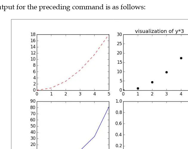
The following figure shows two distributions, binomial and poisson , side by side with various parameters (the visualization was created with matplotlib, which will be covered in Chapter 4, Data Visualization):

Summary

(46)

Chapter 2

Then, we are getting familiar with some common functions and operations on ndarray.

And finally, we continue with some advance functions that are related to statistic, linear algebra and sampling data. Those functions play important role in data analysis.

However, while NumPy by itself does not provide very much high-level data analytical functionality, having an understanding of it will help you use tools such as Pandas much more effectively. This tool will be discussed in the next chapter.

Practice exercises

Exercise 1: Using an array creation function, let's try to create arrays variable in the following situations:

• Create ndarray from the existing data

• Initialize ndarray which elements are filled with ones, zeros, or a given interval

• Loading and saving data from a file to an ndarray

Exercise 2: What is the difference between np.dot(a, b) and (a*b)? Exercise 3: Consider the vector [1, 2, 3, 4, 5] building a new vector with four consecutive zeros interleaved between each value.

Exercise 4: Taking the data example file chapter2-data.txt, which includes information on a system log, solves the following tasks:

• Try to build an ndarray from the data file

• Statistic frequency of each device type in the built matrix • List unique OS that appears in the data log

(47)

(48)

Data Analysis with Pandas

In this chapter, we will explore another data analysis library called Pandas. The goal of this chapter is to give you some basic knowledge and concrete examples for getting started with Pandas.

An overview of the Pandas package

Pandas is a Python package that supports fast, flexible, and expressive data structures, as well as computing functions for data analysis. The following are some prominent features that Pandas supports:

• Data structure with labeled axes. This makes the program clean and clear and avoids common errors from misaligned data.

• Flexible handling of missing data.

• Intelligent label-based slicing, fancy indexing, and subset creation of large datasets.

• Powerful arithmetic operations and statistical computations on a custom axis via axis label.

• Robust input and output support for loading or saving data from and to files, databases, or HDF5 format.

(49)

Data Analysis with Pandas

[ 32 ]

After installation, we can use it like other Python packages. Firstly, we have to import the following packages at the beginning of the program:

>>> import pandas as pd >>> import numpy as np

The Pandas data structure

Let's first get acquainted with two of Pandas' primary data structures: the Series and the DataFrame. They can handle the majority of use cases in finance, statistic, social science, and many areas of engineering.

Series

A Series is a one-dimensional object similar to an array, list, or column in table. Each item in a Series is assigned to an entry in an index:

>>> s1 = pd.Series(np.random.rand(4),

index=['a', 'b', 'c', 'd']) >>> s1

a 0.6122 b 0.98096 c 0.3350 d 0.7221 dtype: float64

By default, if no index is passed, it will be created to have values ranging from 0 to N-1, where N is the length of the Series:

>>> s2 = pd.Series(np.random.rand(4)) >>> s2

(50)

Chapter 3

We can access the value of a Series by using the index:

>>> s1['c'] 0.3350

>>>s1['c'] = 3.14 >>> s1['c', 'a', 'b'] c 3.14

a 0.6122 b 0.98096

This accessing method is similar to a Python dictionary. Therefore, Pandas also allows us to initialize a Series object directly from a Python dictionary:

>>> s3 = pd.Series({'001': 'Nam', '002': 'Mary', '003': 'Peter'})

>>> s3 001 Nam 002 Mary 003 Peter dtype: object

Sometimes, we want to filter or rename the index of a Series created from a Python dictionary. At such times, we can pass the selected index list directly to the initial function, similarly to the process in the above example. Only elements that exist in the index list will be in the Series object. Conversely, indexes that are missing in the dictionary are initialized to default NaN values by Pandas:

>>> s4 = pd.Series({'001': 'Nam', '002': 'Mary', '003': 'Peter'}, index=[ '002', '001', '024', '065']) >>> s4

(51)

[ 34 ]

The library also supports functions that detect missing data:

>>> pd.isnull(s4) 002 False 001 False 024 True 065 True dtype: bool

Similarly, we can also initialize a Series from a scalar value:

>>> s5 = pd.Series(2.71, index=['x', 'y']) >>> s5

x 2.71 y 2.71 dtype: float64

A Series object can be initialized with NumPy objects as well, such as ndarray. Moreover, Pandas can automatically align data indexed in different ways in arithmetic operations:

>>> s6 = pd.Series(np.array([2.71, 3.14]), index=['z', 'y']) >>> s6

z 2.71 y 3.14 dtype: float64 >>> s5 + s6 x NaN y 5.85 z NaN dtype: float64

The DataFrame

The DataFrame is a tabular data structure comprising a set of ordered columns and rows. It can be thought of as a group of Series objects that share an index (the column names). There are a number of ways to initialize a DataFrame object. Firstly, let's take a look at the common example of creating DataFrame from a dictionary of lists:

(52)

Chapter 3

'Density': [244, 256, 268, 279]} >>> df1 = pd.DataFrame(data)

>>> df1

Density Median_Age Year 0 244 24.2 2000 1 256 26.4 2005 2 268 28.5 2010 3 279 30.3 2014

By default, the DataFrame constructor will order the column alphabetically. We can edit the default order by passing the column's attribute to the initializing function:

>>> df2 = pd.DataFrame(data, columns=['Year', 'Density', 'Median_Age']) >>> df2

Year Density Median_Age 0 2000 244 24.2 1 2005 256 26.4 2 2010 268 28.5 3 2014 279 30.3 >>> df2.index

Int64Index([0, 1, 2, 3], dtype='int64')

We can provide the index labels of a DataFrame similar to a Series:

>>> df3 = pd.DataFrame(data, columns=['Year', 'Density', 'Median_Age'], index=['a', 'b', 'c', 'd']) >>> df3.index

Index([u'a', u'b', u'c', u'd'], dtype='object')

We can construct a DataFrame out of nested lists as well:

>>> df4 = pd.DataFrame([

(53)

[ 36 ]

Columns can be accessed by column name as a Series can, either by dictionary-like notation or as an attribute, if the column name is a syntactically valid attribute name:

>>> df4.name # or df4['name'] 0 Peter

1 Mary 2 Nam 3 Mai 4 John

Name: name, dtype: object

To modify or append a new column to the created DataFrame, we specify the column name and the value we want to assign:

>>> df4['award'] = None >>> df4

name age career province sex award 0 Peter 16 pupil TN M None 1 Mary 21 student SG F None 2 Nam 22 student HN M None 3 Mai 31 nurse SG F None 4 John 28 lawer SG M None

Using a couple of methods, rows can be retrieved by position or name:

>>> df4.ix[1] name Mary age 21 career student province SG sex F award None Name: 1, dtype: object

(54)

Chapter 3

Another common case is to provide a DataFrame with data from a location such as a text file. In this situation, we use the read_csv function that expects the column separator to be a comma, by default. However, we can change that by using the sep parameter:

# person.csv file

name,age,career,province,sex Peter,16,pupil,TN,M

Mary,21,student,SG,F Nam,22,student,HN,M Mai,31,nurse,SG,F John,28,lawer,SG,M

# loading person.cvs into a DataFrame >>> df4 = pd.read_csv('person.csv') >>> df4

name age career province sex 0 Peter 16 pupil TN M 1 Mary 21 student SG F 2 Nam 22 student HN M 3 Mai 31 nurse SG F 4 John 28 laywer SG M

While reading a data file, we sometimes want to skip a line or an invalid value. As for Pandas 0.16.2, read_csv supports over 50 parameters for controlling the loading process. Some common useful parameters are as follows:

• sep: This is a delimiter between columns. The default is comma symbol. • dtype: This is a data type for data or columns.

• header: This sets row numbers to use as the column names. • skiprows: This skips line numbers to skip at the start of the file.

• error_bad_lines: This shows invalid lines (too many fields) that will, by default, cause an exception, such that no DataFrame will be returned. If we set the value of this parameter as false, the bad lines will be skipped.

(55)

[ 38 ]

The essential basic functionality

Pandas supports many essential functionalities that are useful to manipulate Pandas data structures. In this book, we will focus on the most important features regarding exploration and analysis.

Reindexing and altering labels

Reindex is a critical method in the Pandas data structures. It confirms whether the new or modified data satisfies a given set of labels along a particular axis of Pandas object.

First, let's view a reindex example on a Series object:

>>> s2.reindex([0, 2, 'b', 3]) 0 0.6913

2 0.8627 b NaN 3 0.7286 dtype: float64

When reindexed labels do not exist in the data object, a default value of NaN will be automatically assigned to the position; this holds true for the DataFrame case as well:

>>> df1.reindex(index=[0, 2, 'b', 3],

columns=['Density', 'Year', 'Median_Age','C']) Density Year Median_Age C

(56)

Chapter 3

We can change the NaN value in the missing index case to a custom value by setting the fill_value parameter. Let us take a look at the arguments that the reindex function supports, as shown in the following table:

Argument Description

index This is the new labels/index to conform to.

method _{This is the method to use for filling holes in a}reindexed object. The default setting is unfill gaps.

pad/ffill: fill values forward

backfill/bfill: fill values backward

nearest: use the nearest value to fill the gap

copy _{This return a new object. The default setting is}true.

level _{The matches index values on the passed multiple index level.} fill_value This is the value to use for missing values. The default setting is

NaN.

limit _{This is the maximum size gap to fill in}forward or backward

method.

Head and tail

In common data analysis situations, our data structure objects contain many columns and a large number of rows. Therefore, we cannot view or load all information of the objects. Pandas supports functions that allow us to inspect a small sample. By default, the functions return five elements, but we can set a custom number as well. The following example shows how to display the first five and the last three rows of a longer Series:

>>> s7 = pd.Series(np.random.rand(10000)) >>> s7.head()

(57)

[ 40 ] dtype: float64

>>> s7.tail(3) 9997 0.412178 9998 0.800711 9999 0.438344 dtype: float64

We can also use these functions for DataFrame objects in the same way.

Binary operations

Firstly, we will consider arithmetic operations between objects. In different indexes objects case, the expected result will be the union of the index pairs. We will not explain this again because we had an example about it in the above section (s5 + s6). This time, we will show another example with a DataFrame:

>>> df5 = pd.DataFrame(np.arange(9).reshape(3,3),0 columns=['a','b','c']) >>> df5

a b c 0 0 1 2 1 3 4 5 2 6 7 8

>>> df6 = pd.DataFrame(np.arange(8).reshape(2,4), columns=['a','b','c','d']) >>> df6

(58)

Chapter 3

The mechanisms for returning the result between two kinds of data structure are similar. A problem that we need to consider is the missing data between objects. In this case, if we want to fill with a fixed value, such as 0, we can use the arithmetic functions such as add, sub, div, and mul, and the function's supported parameters such as fill_value:

>>> df7 = df5.add(df6, fill_value=0) >>> df7

a b c d 0 0 2 4 3 1 7 9 11 7 2 6 7 8 NaN

Next, we will discuss comparison operations between data objects. We have some supported functions such as equal (eq), not equal (ne), greater than (gt), less than (lt), less equal (le), and greater equal (ge). Here is an example:

>>> df5.eq(df6)

a b c d 0 True True True False 1 False False False False 2 False False False False

Functional statistics

The supported statistics method of a library is really important in data analysis. To get inside a big data object, we need to know some summarized information such as mean, sum, or quantile. Pandas supports a large number of methods to compute them. Let's consider a simple example of calculating the sum information of df5, which is a DataFrame object:

Getting Started with Python Data Analysis Learn to use powerful Python libraries for effective data processing and analysis pdf pdf

Getting Started with Python

Data Analysis

Learn to use powerful Python libraries for effective

data processing and analysis

Phuong Vo.T.H

Getting Started with Python Data Analysis

Credits

About the Authors

Phuong Vo.T.H

About the Reviewers

Dong Chao

Hai Minh Nguyen

Kenneth Emeka Odoh

www.PacktPub.com

Support files, eBooks, discount offers, and more

Why subscribe?

Free access for Packt account holders

Table of Contents

Preface v

Chapter 1: Introducing Data Analysis and Libraries

1

Chapter 2: NumPy Arrays and Vectorized Computation

11

Chapter 3: Data Analysis with Pandas

31

Chapter 4: Data Visualization

59

Chapter 5: Time Series

83

Chapter 6: Interacting with Databases

105

Chapter 7: Data Analysis Application Examples

125

Chapter 8: Machine Learning Models with scikit-learn

145

Preface

What this book covers

What you need for this book

Who this book is for

Conventions

Reader feedback

Customer support

Downloading the example code

Errata

Piracy

Questions

Introducing Data Analysis

and Libraries

Data analysis and processing

An overview of the libraries in data

analysis

Python libraries in data analysis

NumPy

Pandas

Matplotlib

PyMongo

The scikit-learn library

Summary

NumPy Arrays and

Vectorized Computation

NumPy arrays

Data types

Array creation

Indexing and slicing

Fancy indexing

Numerical operations on arrays

Array functions

Loading and saving data

Saving an array

Loading an array

Linear algebra with NumPy

NumPy random numbers

Summary

Data Analysis with Pandas

An overview of the Pandas package

The Pandas data structure

Series

The DataFrame

The essential basic functionality