Big Data Analytics with Hadoop 3
Build highly effective analytics solutions to gain valuable insight into your big data
Big Data Analytics with Hadoop 3
Copyright © 2018 Packt Publishing
All rights reserved. No part of this book may be reproduced, stored in a retrieval system, or transmitted in any form or by any means, without the prior written permission of the publisher, except in the case of brief quotations embedded in critical articles or reviews.
Every effort has been made in the preparation of this book to ensure the accuracy of the information presented. However, the information contained in this book is sold without warranty, either express or implied. Neither the authors, nor Packt Publishing or its dealers and distributors, will be held liable for any damages caused or alleged to have been caused directly or indirectly by this book.
Packt Publishing has endeavored to provide trademark information about all of the companies and products mentioned in this book by the appropriate use of capitals. However, Packt Publishing cannot guarantee the accuracy of this information.
Commissioning Editor: Amey Varangaonkar
Acquisition Editor: Varsha Shetty
Content Development Editor: Cheryl Dsa
Technical Editor: Sagar Sawant
Copy Editors: Vikrant Phadke, Safis Editing
Project Coordinator: Nidhi Joshi
Proofreader: Safis Editing
Indexer: Rekha Nair
Graphics: Tania Dutta
Production Coordinator: Arvindkumar Gupta First published: May 2018
mapt.io
Why subscribe?
Spend less time learning and more time coding with practical eBooks and Videos from over 4,000 industry professionals
Improve your learning with Skill Plans built especially for you
Get a free eBook or video every month
Mapt is fully searchable
PacktPub.com
Did you know that Packt offers eBook versions of every book published, with PDF and ePub files available? You can upgrade to the eBook version at www.PacktPub.com and, as a print book customer, you are entitled to a discount on the eBook copy. Get in touch with us at [email protected] for more
details.
About the author
Sridhar Alla is a big data expert helping companies solve complex problems in distributed computing, large scale data science and analytics practice. He presents regularly at several
prestigious conferences and provides training and consulting to companies. He holds a bachelor's in computer science from JNTU, India.
He loves writing code in Python, Scala, and Java. He also has extensive hands-on knowledge of several Hadoop-based technologies, TensorFlow, NoSQL, IoT, and deep learning.
About the reviewers
V. Naresh Kumar has more than a decade of professional experience in designing, implementing, and running very large-scale internet applications in Fortune 500 Companies. He is a full-stack architect with hands-on experience in e-commerce, web hosting, healthcare, big data, analytics, data streaming, advertising, and databases. He admires open source and contributes to it actively. He keeps himself updated with emerging technologies, from Linux system internals to frontend technologies. He studied in BITS- Pilani, Rajasthan, with a joint degree in computer science and economics.
Manoj R. Patil is a big data architect at TatvaSoft—an IT services and consulting firm. He has a bachelor's degree in engineering from COEP, Pune. He is a proven and highly skilled business
intelligence professional with 18 years, experience in IT. He is a seasoned BI and big data consultant with exposure to all the leading platforms.
Previously, he worked for numerous organizations, including Tech Mahindra and Persistent Systems. Apart from authoring a book on Pentaho and big data, he has been an avid reviewer of various titles in the respective fields from Packt and other leading publishers.
Packt is searching for authors like you
Table of Contents
Title PageCopyright and Credits
Big Data Analytics with Hadoop 3 Packt Upsell
Packt is searching for authors like you Preface
Who this book is for What this book covers
To get the most out of this book Download the example code files Download the color images Conventions used
Get in touch Reviews 1. Introduction to Hadoop
Hadoop Distributed File System
Erasure Coding
Intra-DataNode balancer
Installing YARN timeline service v.2 Setting up the HBase cluster
Simple deployment for HBase Enabling the co-processor
Enabling timeline service v.2 Running timeline service v.2
Enabling MapReduce to write to timeline service v.2 Summary
2. Overview of Big Data Analytics Introduction to data analytics
Inside the data analytics process Introduction to big data
Distributed computing using Apache Hadoop The MapReduce framework
Hive
Downloading and extracting the Hive binaries Installing Derby
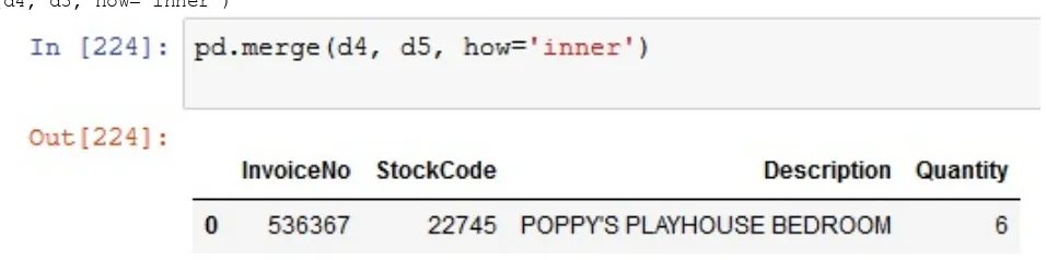
A cheat sheet on retrieving information  Apache Spark
Visualization using Tableau Summary
Shuffle and sort
4. Scientific Computing and Big Data Analysis with Python and Hadoop Installation
5. Statistical Big Data Computing with R and Hadoop Introduction
Install R on workstations and connect to the data in Hadoop Install R on a shared server and connect to Hadoop
Utilize Revolution R Open
Execute R inside of MapReduce using RMR2
Summary and outlook for pure open source options Methods of integrating R and Hadoop
RHADOOP – install R on workstations and connect to data in Hadoop RHIPE – execute R inside Hadoop MapReduce
R and Hadoop Streaming
RHIVE – install R on workstations and connect to data in Hadoop ORCH – Oracle connector for Hadoop
Data analytics Summary
SparkSQL and DataFrames
DataFrame APIs and the SQL API Pivots
Filters
User-defined functions Schema – structure of data
Implicit schema
At-least-once processing
Interoperability with streaming platforms (Apache Kafka) Receiver-based
Direct Stream
Structured Streaming
Getting deeper into Structured Streaming Handling event time and late date
Fault-tolerance semantics Summary
8. Batch Analytics with Apache Flink Introduction to Apache Flink
Continuous processing for unbounded datasets Flink, the streaming model, and bounded datasets Installing Flink
Downloading Flink Installing Flink
Starting a local Flink cluster Using the Flink cluster UI
Batch analytics Reading file
Transformations
9. Stream Processing with Apache Flink
Introduction to streaming execution model Data processing using the DataStream API
Elasticsearch connector Cassandra connector Summary
10. Visualizing Big Data Introduction
Using Python to visualize data Using R to visualize data Big data visualization tools Summary
11. Introduction to Cloud Computing Concepts and terminology
Cloud IT resource On-premise
Resiliency
12. Using Amazon Web Services
Amazon Elastic Compute Cloud
Instances and Amazon Machine Images Launching multiple instances of an AMI
Instances AMIs
Regions and availability zones
Region and availability zone concepts Regions
Amazon EC2 security groups for Linux instances Elastic IP addresses
Amazon EC2 and Amazon Virtual Private Cloud Amazon Elastic Block Store
Amazon EC2 instance store What is AWS Lambda?
When should I use AWS Lambda? Introduction to Amazon S3
Getting started with Amazon S3
Flexible management
Most supported platform with the largest ecosystem Easy and flexible data transfer
Backup and recovery Data archiving
Data lakes and big data analytics Hybrid Cloud storage
Cloud-native application data Disaster recovery
Amazon DynamoDB
Amazon Kinesis Data Streams
What can I do with Kinesis Data Streams?
Accelerated log and data feed intake and processing Real-time metrics and reporting
Real-time data analytics Complex stream processing
Benefits of using Kinesis Data Streams AWS Glue
When should I use AWS Glue? Amazon EMR
Preface
Apache Hadoop is the most popular platform for big data processing, and can be combined with a host of other big data tools to build powerful analytics solutions. Big Data Analytics with Hadoop 3
shows you how to do just that, by providing insights into the software as well as its benefits with the help of practical examples.
Once you have taken a tour of Hadoop 3's latest features, you will get an overview of HDFS, MapReduce, and YARN, and how they enable faster, more efficient big data processing. You will then move on to learning how to integrate Hadoop with open source tools, such as Python and R, to analyze and visualize data and perform statistical computing on big data. As you become acquainted with all of this, you will explore how to use Hadoop 3 with Apache Spark and Apache Flink for real-time data analytics and stream processing. In addition to this, you will understand how to use Hadoop to build analytics solutions in the cloud and an end-to-end pipeline to perform big data analysis using practical use cases.
By the end of this book, you will be well-versed with the analytical capabilities of the Hadoop
Who this book is for
Big Data Analytics with Hadoop 3 is for you if you are looking to build high-performance analytics
What this book covers
Chapter 1, Introduction to Hadoop, introduces you to the world of Hadoop and its core components, namely, HDFS and MapReduce.
Chapter 2, Overview of Big Data Analytics, introduces the process of examining large datasets to uncover patterns in data, generating reports, and gathering valuable insights.
Chapter 3, Big Data Processing with MapReduce, introduces the concept of MapReduce, which is the fundamental concept behind most of the big data computing/processing systems.
Chapter 4, Scientific Computing and Big Data Analysis with Python and Hadoop, provides an introduction to Python and an analysis of big data using Hadoop with the aid of Python packages.
Chapter 5, Statistical Big Data Computing with R and Hadoop, provides an introduction to R and demonstrates how to use R to perform statistical computing on big data using Hadoop.
Chapter 6, Batch Analytics with Apache Spark, introduces you to Apache Spark and demonstrates how to use Spark for big data analytics based on a batch processing model.
Chapter 7, Real-Time Analytics with Apache Spark, introduces the stream processing model of Apache Spark and demonstrates how to build streaming-based, real-time analytical applications.
Chapter 8, Batch Analytics with Apache Flink, covers Apache Flink and how to use it for big data analytics based on a batch processing model.
Chapter 9, Stream Processing with Apache Flink, introduces you to DataStream APIs and stream processing using Flink. Flink will be used to receive and process real-time event streams and store the aggregates and results in a Hadoop cluster.
Chapter 10, Visualizing Big Data, introduces you to the world of data visualization using various tools and technologies such as Tableau.
Chapter 11, Introduction to Cloud Computing, introduces Cloud computing and various concepts such as IaaS, PaaS, and SaaS. You will also get a glimpse into the top Cloud providers.
To get the most out of this book
The examples have been implemented using Scala, Java, R, and Python on a Linux 64-bit. You will also need, or be prepared to install, the following on your machine (preferably the latest version):
Spark 2.3.0 (or higher) Hadoop 3.1 (or higher) Flink 1.4
Java (JDK and JRE) 1.8+ Scala 2.11.x (or higher) Python 2.7+/3.4+
R 3.1+ and RStudio 1.0.143 (or higher) Eclipse Mars or Idea IntelliJ (latest)
Regarding the operating system: Linux distributions are preferable (including Debian, Ubuntu, Fedora, RHEL, and CentOS) and, to be more specific, for example, as regards Ubuntu, it is
recommended having a complete 14.04 (LTS) 64-bit (or later) installation, VMWare player 12, or Virtual box. You can also run code on Windows (XP/7/8/10) or macOS X (10.4.7+).
Download the example code files
You can download the example code files for this book from your account at www.packtpub.com. If you purchased this book elsewhere, you can visit www.packtpub.com/support and register to have the files emailed directly to you.
You can download the code files by following these steps: 1. Log in or register at www.packtpub.com.
2. Select the SUPPORT tab.
3. Click on Code Downloads & Errata.
4. Enter the name of the book in the Search box and follow the onscreen instructions.
Once the file is downloaded, please make sure that you unzip or extract the folder using the latest version of:
WinRAR/7-Zip for Windows Zipeg/iZip/UnRarX for Mac 7-Zip/PeaZip for Linux
The code bundle for the book is also hosted on GitHub at https://github.com/PacktPublishing/Big-Data-Analy tics-with-Hadoop-3. In case there's an update to the code, it will be updated on the existing GitHub
repository.
Download the color images
Conventions used
There are a number of text conventions used throughout this book.
CodeInText: Indicates code words in text, database table names, folder names, filenames, file
extensions, pathnames, dummy URLs, user input, and Twitter handles. Here is an example: "This file, temperatures.csv, is available as a download and once downloaded, you can move it into hdfs by running the command, as shown in the following code."
A block of code is set as follows:
hdfs dfs -copyFromLocal temperatures.csv /user/normal
When we wish to draw your attention to a particular part of a code block, the relevant lines or items are set in bold:
Map-Reduce Framework -- output average temperature per city name
Map input records=35 Map output records=33
Map output bytes=208
Map output materialized bytes=286
Any command-line input or output is written as follows:
$ ssh-keygen -t rsa -P '' -f ~/.ssh/id_rsa
$ cat ~/.ssh/id_rsa.pub >> ~/.ssh/authorized_keys $ chmod 0600 ~/.ssh/authorized_keys
Bold: Indicates a new term, an important word, or words that you see on screen. For example, words in menus or dialog boxes appear in the text like this. Here is an example: "Clicking on
the Datanodes tab shows all the nodes."
Warnings or important notes appear like this.
Get in touch
Feedback from our readers is always welcome.
General feedback: Email [email protected] and mention the book title in the subject of your
message. If you have questions about any aspect of this book, please email us at [email protected].
Errata: Although we have taken every care to ensure the accuracy of our content, mistakes do
happen. If you have found a mistake in this book, we would be grateful if you would report this to us. Please visit www.packtpub.com/submit-errata, selecting your book, clicking on the Errata Submission Form link, and entering the details.
Piracy: If you come across any illegal copies of our works in any form on the Internet, we would be grateful if you would provide us with the location address or website name. Please contact us at [email protected] with a link to the material.
Reviews
Please leave a review. Once you have read and used this book, why not leave a review on the site that you purchased it from? Potential readers can then see and use your unbiased opinion to make purchase decisions, we at Packt can understand what you think about our products, and our authors can see your feedback on their book. Thank you!
Introduction to Hadoop
This chapter introduces the reader to the world of Hadoop and the core components of Hadoop, namely the Hadoop Distributed File System (HDFS) and MapReduce. We will start by introducing the changes and new features in the Hadoop 3 release. Particularly, we will talk about the new
features of HDFS and Yet Another Resource Negotiator (YARN), and changes to client
applications. Furthermore, we will also install a Hadoop cluster locally and demonstrate the new features such as erasure coding (EC) and the timeline service. As as quick note, Chapter
10, Visualizing Big Data shows you how to create a Hadoop cluster in AWS.
Hadoop Distributed File System
HDFS is a software-based filesystem implemented in Java and it sits on top of the native filesystem. The main concept behind HDFS is that it divides a file into blocks (typically 128 MB) instead of dealing with a file as a whole. This allows many features such as distribution, replication, failure recovery, and more importantly distributed processing of the blocks using multiple machines. Block sizes can be 64 MB, 128 MB, 256 MB, or 512 MB, whatever suits the purpose. For a 1 GB file with 128 MB blocks, there will be 1024 MB/128 MB equal to eight blocks. If you consider a replication factor of three, this makes it 24 blocks. HDFS provides a distributed storage system with fault
tolerance and failure recovery. HDFS has two main components: the NameNode and the DataNode. The NameNode contains all the metadata of all content of the filesystem: filenames, file permissions, and the location of each block of each file, and hence it is the most important machine in HDFS. DataNodes connect to the NameNode and store the blocks within HDFS. They rely on the NameNode for all metadata information regarding the content in the filesystem. If the NameNode does not have any information, the DataNode will not be able to serve information to any client who wants to read/write to the HDFS.
It is possible for NameNode and DataNode processes to be run on a single machine; however, generally HDFS clusters are made up of a dedicated server running the NameNode process and thousands of machines running the DataNode process. In order to be able to access the content
information stored in the NameNode, it stores the entire metadata structure in memory. It ensures that there is no data loss as a result of machine failures by keeping a track of the replication factor of blocks. Since it is a single point of failure, to reduce the risk of data loss on account of the failure of a NameNode, a secondary NameNode can be used to generate snapshots of the primary NameNode's memory structures.
DataNodes have large storage capacities and, unlike the NameNode, HDFS will continue to operate normally if a DataNode fails. When a DataNode fails, the NameNode automatically takes care of the now diminished replication of all the data blocks in the failed DataNode and makes sure the
replication is built back up. Since the NameNode knows all locations of the replicated blocks, any clients connected to the cluster are able to proceed with little to no hiccups.
In order to make sure that each block meets the minimum required replication factor, the NameNode replicates the lost blocks.
High availability
The loss of NameNodes can crash the cluster in both Hadoop 1.x as well as Hadoop 2.x. In Hadoop 1.x, there was no easy way to recover, whereas Hadoop 2.x introduced high availability (active-passive setup) to help recover from NameNode failures.
The following diagram shows how high availability works:
In Hadoop 3.x you can have two passive NameNodes along with the active node, as well as five
JournalNodes to assist with recovery from catastrophic failures:
NameNode machines: The machines on which you run the active and standby NameNodes. They should have equivalent hardware to each other and to what would be used in a non-HA cluster.
JournalNode machines: The machines on which you run the JournalNodes. The JournalNode daemon is relatively lightweight, so these daemons may reasonably be collocated on machines with other Hadoop daemons, for example NameNodes, the JobTracker, or the YARN
Intra-DataNode balancer
HDFS has a way to balance the data blocks across the data nodes, but there is no such balancing inside the same data node with multiple hard disks. Hence, a 12-spindle DataNode can have out of balance physical disks. But why does this matter to performance? Well, by having out of balance disks, the blocks at DataNode level might be the same as other DataNodes but the reads/writes will be skewed because of imbalanced disks. Hence, Hadoop 3.x introduces the intra-node balancer to balance the physical disks inside each data node to reduce the skew of the data.
This increases the reads and writes performed by any process running on the cluster, such as a
Erasure coding
HDFS has been the fundamental component since the inception of Hadoop. In Hadoop 1.x as well as Hadoop 2.x, a typical HDFS installation uses a replication factor of three.
Compared to the default replication factor of three, EC is probably the biggest change in HDFS in years and fundamentally doubles the capacity for many datasets by bringing down the replication factor from 3 to about 1.4. Let's now understand what EC is all about.
EC is a method of data protection in which data is broken into fragments, expanded, encoded with redundant data pieces, and stored across a set of different locations or storage. If at some point during this process data is lost due to corruption, then it can be reconstructed using the information stored elsewhere. Although EC is more CPU intensive, this greatly reduces the storage needed for the
Port numbers
In Hadoop 3.x, many of the ports for various services have been changed.
Previously, the default ports of multiple Hadoop services were in the Linux ephemeral port range (32768–61000). This indicated that at startup, services would sometimes fail to bind to the port with another application due to a conflict.
These conflicting ports have been moved out of the ephemeral range, affecting the NameNode, Secondary NameNode, DataNode, and KMS.
The changes are listed as follows:
NameNode ports: 50470 → 9871, 50070 → 9870, and 8020 → 9820
Secondary NameNode ports: 50091 → 9869 and 50090 → 9868
MapReduce framework
Task-level native optimization
MapReduce has added support for a native implementation of the map output collector. This new support can result in a performance improvement of about 30% or more, particularly for shuffle-intensive jobs.
The native library will build automatically with Pnative. Users may choose the new collector on a job-by-job basis by setting mapreduce.job.map.output.collector.class=org.apache.hadoop.mapred.
nativetask.NativeMapOutputCollectorDelegator in their job configuration.
The basic idea is to be able to add a NativeMapOutputCollector in order to handle key/value pairs emitted by mapper. As a result of this sort, spill, and IFile serialization can all be done in native code. A preliminary test (on Xeon E5410, jdk6u24) showed promising results as follows:
sort is about 3-10 times faster than Java (only binary string compare is supported)
IFile serialization speed is about three times faster than Java: about 500 MB per second. If
YARN
When an application wants to run, the client launches the ApplicationMaster, which then negotiates with the ResourceManager to get resources in the cluster in the form of containers. A container represents CPUs (cores) and memory allocated on a single node to be used to run tasks and
processes. Containers are supervised by the NodeManager and scheduled by the ResourceManager.
Examples of containers:
One core and 4 GB RAM Two cores and 6 GB RAM Four cores and 20 GB RAM
Some containers are assigned to be mappers and others to be reducers; all this is coordinated by the ApplicationMaster in conjunction with the ResourceManager. This framework is called YARN:
Using YARN, several different applications can request for and execute tasks on containers, sharing the cluster resources pretty well. However, as the size of the clusters grows and the variety of
Opportunistic containers
Opportunistic containers can be transmitted to a NodeManager even if their execution at that
particular time cannot begin immediately, unlike YARN containers, which are scheduled in a node if and only if there are unallocated resources.
Types of container execution
There are two types of container, as follows:Guaranteed containers: These containers correspond to the existing YARN containers. They are assigned by the capacity scheduler. They are transmitted to a node if and only if there are resources available to begin their execution immediately.
YARN timeline service v.2
The YARN timeline service v.2 addresses the following two major challenges: Enhancing the scalability and reliability of the timeline service
Enhancing scalability and reliability
Version 2 adopts a more scalable distributed writer architecture and backend storage, as opposed to v.1 which does not scale well beyond small clusters as it used a single instance of writer/reader architecture and backend storage.
Usability improvements
Many a time, users are more interested in the information obtained at the level of flows or in logical groups of YARN applications. For this reason, it is more convenient to launch a series of YARN applications to complete a logical workflow.
Architecture
YARN Timeline Service v.2 uses a set of collectors (writers) to write data to the back-end storage. The collectors are distributed and co-located with the application masters to which they are dedicated. All data that belong to that application are sent to the application level timeline collectors with the exception of the resource manager timeline collector.
For a given application, the application master can write data for the application to the co-located timeline collectors (which is an NM auxiliary service in this release). In addition, node managers of other nodes that are running the containers for the application also write data to the timeline collector on the node that is running the application master.
The resource manager also maintains its own timeline collector. It emits only YARN-generic life-cycle events to keep its volume of writes reasonable.
Other changes
There are other changes coming up in Hadoop 3, which are mainly to make it easier to maintain and operate. Particularly, the command-line tools have been revamped to better suit the needs of
Minimum required Java version
Shell script rewrite
The Hadoop shell scripts have been rewritten to fix many long-standing bugs and include some new features.
Incompatible changes are documented in the release notes. You can find them at https://issues.apache.or g/jira/browse/HADOOP-9902.
Shaded-client JARs
The new hadoop-client-api and hadoop-client-runtime artifacts have been added, as referred to by https://is sues.apache.org/jira/browse/HADOOP-11804. These artifacts shade Hadoop's dependencies into a single JAR. As a result, it avoids leaking Hadoop's dependencies onto the application's classpath.
Installing Hadoop 3
In this section, we shall see how to install a single-node Hadoop 3 cluster on your local machine. In order to do this, we will be following the documentation given at https://hadoop.apache.org/docs/current/h adoop-project-dist/hadoop-common/SingleCluster.html.
Prerequisites
Java 8 must be installed for Hadoop to be run. If Java 8 does not exist on your machine, then you can download and install Java 8: https://www.java.com/en/download/.
Downloading
Download the Hadoop 3.1 version using the following link: http://apache.spinellicreations.com/hadoop/com mon/hadoop-3.1.0/.
The following screenshot is the page shown when the download link is opened in the browser:
Installation
Perform the following steps to install a single-node Hadoop cluster on your machine: 1. Extract the downloaded file using the following command:
tar -xvzf hadoop-3.1.0.tar.gz
2. Once you have extracted the Hadoop binaries, just run the following commands to test the Hadoop binaries and make sure the binaries works on our local machine:
cd hadoop-3.1.0
mkdir input
cp etc/hadoop/*.xml input
bin/hadoop jar share/hadoop/mapreduce/hadoop-mapreduce-examples-3.1.0.jar grep input output 'dfs[a-z.]+'
cat output/*
If everything runs as expected, you will see an output directory showing some output, which shows that the sample command worked.
Setup password-less ssh
Now check if you can ssh to the localhost without a passphrase by running a simple command, shown as follows:
$ ssh localhost
If you cannot ssh to localhost without a passphrase, execute the following commands:
$ ssh-keygen -t rsa -P '' -f ~/.ssh/id_rsa
Setting up the NameNode
Make the following changes to the configuration file etc/hadoop/core-site.xml:
<configuration> <property>
<name>fs.defaultFS</name>
<value>hdfs://localhost:9000</value> </property>
</configuration>
Make the following changes to the configuration file etc/hadoop/hdfs-site.xml:
<configuration> <property>
<name>dfs.replication</name> <value>1</value>
</property>
<name>dfs.name.dir</name>
<value><YOURDIRECTORY>/hadoop-3.1.0/dfs/name</value> </property>
Starting HDFS
Follow these steps as shown to start HDFS (NameNode and DataNode): 1. Format the filesystem:
$ ./bin/hdfs namenode -format
2. Start the NameNode daemon and the DataNode daemon:
$ ./sbin/start-dfs.sh
The Hadoop daemon log output is written to the $HADOOP_LOG_DIR directory (defaults to $HADOOP_HOME/logs).
3. Browse the web interface for the NameNode; by default it is available at http://localhost:9870/. 4. Make the HDFS directories required to execute MapReduce jobs:
$ ./bin/hdfs dfs -mkdir /user
$ ./bin/hdfs dfs -mkdir /user/<username>
5. When you're done, stop the daemons with the following:
$ ./sbin/stop-dfs.sh
6. Open a browser to check your local Hadoop, which can be launched in the
Figure: Screenshot showing the nodes in the Datanodes tab
8. Clicking on the logs will show the various logs in your cluster, as shown in the following screenshot:
Figure: Screenshot showing the Browse Directory and how you can browse the filesystem in you newly installed cluster
Setting up the YARN service
In this section, we will set up a YARN service and start the components needed to run and operate a YARN cluster:
1. Start the ResourceManager daemon and the NodeManager daemon:
$ sbin/start-yarn.sh
2. Browse the web interface for the ResourceManager; by default it is available at: http://localhost:8088/
3. Run a MapReduce job
4. When you're done, stop the daemons with the following:
$ sbin/stop-yarn.sh
Figure: Screenshot of YARN ResouceManager
Figure: Screenshot of queues of resources in the cluster
Erasure Coding
EC is a key change in Hadoop 3.x promising a significant improvement in HDFS utilization efficiencies as compared to earlier versions where replication factor of 3 for instance caused immense wastage of precious cluster file system for all kinds of data no matter what the relative importance was to the tasks at hand.
EC can be setup using policies and assigning the policies to directories in HDFS. For this, HDFS provides an ec subcommand to perform administrative commands related to EC:
hdfs ec [generic options]
[-setPolicy -path <path> [-policy <policyName>] [-replicate]] [-getPolicy -path <path>]
[-unsetPolicy -path <path>] [-listPolicies]
[-addPolicies -policyFile <file>] [-listCodecs]
[-enablePolicy -policy <policyName>] [-disablePolicy -policy <policyName>] [-help [cmd ...]]
The following are the details of each command:
[-setPolicy -path <path> [-policy <policyName>] [-replicate]]: Sets an EC policy on a directory at the specified path.
path: An directory in HDFS. This is a mandatory parameter. Setting a policy only affects newly created files, and does not affect existing files.
policyName: The EC policy to be used for files under this
directory. This parameter can be omitted if a dfs.namenode.ec.system.default.policy configuration is set. The EC policy of the path will be set with the default value in configuration.
-replicate: Apply the special REPLICATION policy on the directory, force the directory to
adopt 3x replication scheme.
-replicate and -policy <policyName>: These are optional arguments. They cannot be specified at the same time.
[-getPolicy -path <path>]: Get details of the EC policy of a file or directory at the specified path.
[-unsetPolicy -path <path>]: Unset an EC policy set by a previous call to setPolicy on a directory. If the directory inherits the EC policy from an ancestor directory, unsetPolicy is a no-op. Unsetting the policy on a directory which doesn't have an explicit policy set will not return an error.
[-listPolicies]: Lists all (enabled, disabled and removed) EC policies
registered in HDFS. Only the enabled policies are suitable for use with the setPolicy command. [-addPolicies -policyFile <file>]: Add a list of EC policies. Please refer
etc/hadoop/user_ec_policies.xml.template for the example policy file. The maximum cell size is defined in property
dfs.namenode.ec.policies.max.cellsize with the default value 4 MB.
of 64 to 127. Adding policy will fail if there are already 64 policies added.
[-listCodecs]: Get the list of supported EC codecs and coders in system. A
coder is an implementation of a codec. A codec can have different implementations, thus different coders. The coders for a codec are listed in a fall
back order.
[-removePolicy -policy <policyName>]: It removes an EC policy [-enablePolicy -policy <policyName>]: It enables an EC policy [-disablePolicy -policy <policyName>]: It disables an EC policy
Lets test out EC in our cluster. First we will create directories in the HDFS shown as follows: ./bin/hdfs dfs -mkdir /user/normal
./bin/hdfs dfs -mkdir /user/ec
Once the two directories are created then you can set the policy on any path:
./bin/hdfs ec -setPolicy -path /user/ec -policy RS-6-3-1024k Set RS-6-3-1024k erasure coding policy on /user/ec
Type the command shown as follows to test this:
./bin/hdfs dfs -copyFromLocal ~/Documents/OnlineRetail.csv /user/ec
Intra-DataNode balancer
While HDFS always had a great feature of balancing the data between the data nodes in the cluster, often this resulted in skewed disks within data nodes. For instance, if you have four disks, two disks might take the bulk of the data and the other two might be under-utilized. Given that physical disks (say 7,200 or 10,000 rpm) are slow to read/write, this kind of skewing of data results in poor performance. Using an intra-node balancer, we can rebalance the data amongst the disks.
Run the command shown in the following example to invoke disk balancing on a DataNode:
./bin/hdfs diskbalancer -plan 10.0.0.103
Installing YARN timeline service v.2
As stated in the YARN timeline service v.2 section, v.2 always selects Apache HBase as the primary backing storage, since Apache HBase scales well even to larger clusters and continues to maintain a good read and write response time.
There are a few steps that need to be performed to prepare the storage for timeline service v.2: 1. Set up the HBase cluster
2. Enable the co-processor
3. Create the schema for timeline service v.2
Setting up the HBase cluster
Simple deployment for HBase
If you are intent on a simple deploy profile for the Apache HBase cluster where the data loading is light but the data needs to persist across node comings and goings, you could consider the Standalone HBase over HDFS deploy mode.
http://mirror.cogentco.com/pub/apache/hbase/1.2.6/
Download hbase-1.2.6-bin.tar.gz to your local machine. Then extract the HBase binaries:
tar -xvzf hbase-1.2.6-bin.tar.gz
The following is the content of the extracted HBase:
This is a useful variation on the standalone HBase setup and has all HBase daemons running inside one JVM but rather than persisting to the local filesystem, it persists to an HDFS instance. Writing to HDFS where data is replicated ensures that data is persisted across node comings and goings. To configure this standalone variant, edit your hbasesite.xml setting the hbase.rootdir to point at a directory in your HDFS instance but then set hbase.cluster.distributed to false.
The following is the hbase-site.xml with the hdfs port 9000 for the local cluster we have installed mentioned as a property. If you leave this out there wont be a HBase cluster installed.
<configuration> <property>
<name>hbase.rootdir</name>
<value>hdfs://localhost:9000/hbase</value> </property>
<property>
<name>hbase.cluster.distributed</name> <value>false</value>
</property> </configuration>
Next step is to start HBase. We will do this by using start-hbase.sh script:
./bin/start-hbase.sh
Figure: Screenshot of attributes of the HBase cluster setup and the versions of different components
Enabling the co-processor
In this version, the co-processor is loaded dynamically.Copy the timeline service .jar to HDFS from where HBase can load it. It is needed for the flowrun table creation in the schema creator. The default HDFS location is /hbase/coprocessor.
For example:
hadoop fs -mkdir /hbase/coprocessor hadoop fs -put hadoop-yarn-server-timelineservice-hbase-3.0.0-alpha1-SNAPSHOT.jar /hbase/coprocessor/hadoop-yarn-server-timelineservice.jar
To place the JAR at a different location on HDFS, there also exists a YARN configuration setting called yarn.timeline-service.hbase.coprocessor.jar.hdfs.location, shown as follows:
<property>
<name>yarn.timeline-service.hbase.coprocessor.jar.hdfs.location</name> <value>/custom/hdfs/path/jarName</value>
</property>
Create the timeline service schema using the schema creator tool. For this to happen, we also need to make sure the JARs are all found correctly:
export HADOOP_CLASSPATH=$HADOOP_CLASSPATH:/Users/sridharalla/hbase-1.2.6/lib/:/Users/sridharalla/hadoop-3.1.0/share/hadoop/yarn/timelineservice/
Once we have the classpath corrected, we can create the HBase schema/tables using a simple command, shown as follows:
./bin/hadoop org.apache.hadoop.yarn.server.timelineservice.storage.TimelineSchemaCreator -create -skipExistingTable
Enabling timeline service v.2
The following are the basic configurations to start timeline service v.2:
<property>
<description> This setting indicates if the yarn system metrics is published by RM and NM by on the timeline service. </description> <name>yarn.system-metrics-publisher.enabled</name>
<value>true</value> </property>
<property>
<description>This setting is to indicate if the yarn container events are published by RM to the timeline service or not. This configuration is for ATS V2. </description> <name>yarn.rm.system-metrics-publisher.emit-container-events</name>
<value>true</value> </property>
Also, add the hbase-site.xml configuration file to the client Hadoop cluster configuration so that it can write data to the Apache HBase cluster you are using, or set
yarn.timeline-service.hbase.configuration.file to the file URL pointing to hbase-site.xml for the same purpose of writing the data to HBase, for example:
<property>
<description>This is an Optional URL to an hbase-site.xml configuration file. It is to be used to connect to the timeline-service hbase cluster. If it is empty or not specified, the HBase configuration will be loaded from the classpath. Else, they will override those from the ones present on the classpath. </description> <name>yarn.timeline-service.hbase.configuration.file</name>
Running timeline service v.2
Restart the ResourceManager as well as the node managers to pick up the new configuration. The collectors start within the resource manager and the node managers in an embedded manner.
The timeline service reader is a separate YARN daemon, and it can be started using the following syntax:
Enabling MapReduce to write to timeline
service v.2
To write MapReduce framework data to timeline service v.2, enable the following configuration in mapred-site.xml:
<property>
<name>mapreduce.job.emit-timeline-data</name> <value>true</value>
</property>
Summary
In this chapter, we have discussed the new features in Hadoop 3.x and how it improves the reliability and performance of Hadoop 2.x. We also walked through the installation of a standalone Hadoop cluster on the local machine.
Overview of Big Data Analytics
In this chapter, we will talk about big data analytics, starting with a general point of view and then taking a deep dive into some common technologies used to gain insights into data. This chapter introduces the reader to the process of examining large data sets to uncover patterns in data,
generating reports, and gathering valuable insights. We will particularly focus on the seven Vs of big data. We will also learn about data analysis and big data; we will see the challenges that big data provides and how they are dealt with in distributed computing, and look at approaches using Hive and Tableau to showcase the most commonly used technologies.
In a nutshell, the following topics will be covered throughout this chapter: Introduction to data analytics
Introduction to big data
Distributed computing using Apache Hadoop MapReduce framework
Hive
Introduction to data analytics
Data analytics is the process of applying qualitative and quantitative techniques when examining data, with the goal of providing valuable insights. Using various techniques and concepts, data analytics can provide the means to explore the data exploratory data analysis (EDA) as well as draw
conclusions about the data confirmatory data analysis (CDA). The EDA and CDA are fundamental concepts of data analytics, and it is important to understand the differences between the two.
Inside the data analytics process
Once data is deemed ready, it can be analyzed and explored by data scientists using statistical methods such as SAS. Data governance also becomes a factor to ensure the proper collection and protection of the data. Another less well known role is that of a data steward who specializes in understanding the data to the byte; exactly where it is coming from, all transformations that occur, and what the business really needs from the column or field of data.
Various entities in the business might be dealing with addresses differently, such as the following:
123 N Main St vs 123 North Main Street.
But, our analytics depend on getting the correct address field, else both the addresses mentioned will be considered different and our analytics will not have the same accuracy.
The analytics process starts with data collection based on what the analysts might need from the data warehouse, collecting all sorts of data in the organization (sales, marketing, employee, payroll, HR, and so on). Data stewards and governance teams are important here to make sure the right data is collected and that any information deemed confidential or private is not accidentally exported out, even if the end users are all employees. Social Security Numbers (SSNs) or full addresses might not be a good idea to include in analytics as this can cause a lot of problems to the organization.
Data quality processes must be established to make sure that the data being collected and engineered is correct and will match the needs of the data scientists. At this stage, the main goal is to find and fix data quality problems that could affect the accuracy of analytical needs. Common techniques are profiling the data, cleansing the data to make sure that the information in a dataset is consistent, and also that any errors and duplicate records are removed.
Analytical applications can thus be realized using several disciplines, teams, and skillsets. Analytical applications can be used to generate reports all the way to automatically triggering business actions. For example, you can simply a create daily sales report to be emailed out to all managers every day at 8 AM in the morning. But, you can also integrate with business process management applications or some custom stock trading applications to take action, such as buying, selling, or alerting on activities in the stock market. You can also think of taking in news articles or social media information to
further influence what decisions to be made.
Data visualization is an important piece of data analytics and it's hard to understand numbers when you are looking at a lot of metrics and calculation. Rather, there is an increasing dependence on
business intelligence (BI) tools, such as Tableau, QlikView, and so on, to explore and analyze the data. Of course, large-scale visualization, such as showing all Uber cars in the country or heat maps showing water supply in New York City, requires more custom applications or specialized tools to be built.
sizes across all industries. Businesses have always struggled to find a pragmatic approach to capturing information about their customers, products, and services. When the company only had a handful of customers who bought a few of their items, it was not that difficult. It was not as big of a challenge. But over time, companies in the markets started growing. Things have become more
complicated. Now, we have branding information and social media. We have things that are sold and bought over the internet. We need to come up with different solutions. With web development,
Introduction to big data
Twitter, Facebook, Amazon, Verizon, Macy's, and Whole Foods are all companies that run their business using data analytics and base many of the decisions on the analytics. Think about what kind of data they are collecting, how much data they might be collecting, and then how they might be using the data.
Let's look at the grocery store example seen earlier; what if the store starts expanding its business to set up hundreds of stores? Naturally, the sales transactions will have to be collected and stored at a scale hundreds of times more than the single store. But then, no business works independently any more. There is a lot of information out there, starting from local news, tweets, Yelp reviews,
customer complaints, survey activities, competition from other stores, the changing demographics or economy of the local area, and so on. All such additional data can help in better understanding the customer behavior and the revenue models.
For example, if we see increasing negative sentiment regarding the store's parking facility, then we could analyze this and take corrective action such as validated parking or negotiating with the city's public transportation department to provide more frequent trains or buses for better reach. Such an increasing quantity and variety of data, while it provides better analytics also poses challenges to the business IT organization trying to store and process and analyze all the data. It is, in fact, not
uncommon to see TBs of data.
Every day, we create more than two quintillion bytes of data (2 EB), and it is estimated that more than 90% of the data has been generated in last few years alone:
1 KB = 1024 Bytes 1 MB = 1024 KB 1 GB = 1024 MB
1 TB = 1024 GB ~ 1,000,000 MB
1 PB = 1024 TB ~ 1,000,000 GB ~ 1,000,000,000 MB
1 EB = 1024 PB ~ 1,000,000 TB ~ 1,000,000,000 GB ~ 1,000,000,000,000 MB
Such large amounts of data since the 1990s and the need to understand and make sense of the data, gave rise to the term big data.
In 2001, Doug Laney, then an analyst at consultancy Meta Group Inc (which got acquired by Gartner), introduced the idea of three Vs (that is, Variety, Velocity, and Volume). Now, we refer to four Vs instead of three Vs with the addition of Veracity of data to the three Vs.
Variety of data
Velocity of data
Data can be from a data warehouse, batch mode file archives, near real-time updates, or
Volume of data
Veracity of data
Data can be analyzed for actionable insights, but with so much data of all types being analyzed from across data sources, it is very difficult to ensure correctness and proof of accuracy.
The following are the four Vs of big data:
To make sense of all the data and apply data analytics to big data, we need to expand the concept of data analytics to operate at a much larger scale that deals with the four Vs of big data. This changes not only the tools and technologies and methodologies used in analyzing the data, but also changes the way we even approach the problem. If a SQL database was used for data in a business in 1999, to handle the data now for the same business, we will need a distributed SQL database that is scalable and adaptable to the nuances of the big data space.
Variability of data
Visualization
Value
Distributed computing using Apache Hadoop
We are surrounded by devices such as the smart refrigerator, smart watch, phone, tablet, laptops, kiosks at the airport, ATMs dispensing cash to you, and many many more, with the help of which we are now able to do things that were unimaginable just a few years ago. We are so used to applications such as Instagram, Snapchat, Gmail, Facebook, Twitter, and Pinterest that it is next to impossible to go a day without access to such applications. Today, cloud computing has introduced us to the following concepts:Infrastructure as a Service Platform as a Service Software as a Service
Behind the scenes is the world of highly scalable distributed computing, which makes it possible to store and process Petabytes (PB) of data:
1 EB = 1024 PB (50 million Blu-ray movies) 1 PB = 1024 TB (50,000 Blu-ray movies) 1 TB = 1024 GB (50 Blu-ray movies)
The average size of one Blu-ray disc for a movie is ~ 20 GB.
Now, the paradigm of distributed computing is not really a genuinely new topic and has been pursued in some shape or form over decades, primarily at research facilities as well as by a few commercial product companies. Massively parallel processing (MPP) is a paradigm that was in use decades ago in several areas such as oceanography, earthquake monitoring, and space exploration. Several
companies, such as Teradata, also implemented MPP platforms and provided commercial products and applications.
Eventually, tech companies such as Google and Amazon, among others, pushed the niche area of scalable distributed computing to a new stage of evolution, which eventually led to the creation of Apache Spark by Berkeley University. Google published a paper on MapReduce as well as Google File System (GFS), which brought the principles of distributed computing to be used by everyone. Of course, due credit needs to be given to Doug Cutting, who made it possible by implementing the concepts given in the Google white papers and introducing the world to Hadoop. The Apache Hadoop framework is an open source software framework written in Java. The two main areas provided by the framework are storage and processing. For storage, the Apache Hadoop framework uses Hadoop Distributed File System (HDFS), which is based on the GFS paper released on
The MapReduce framework
MapReduce is a framework used to compute a large amount of data in a Hadoop cluster. MapReduce uses YARN to schedule the mappers and reducers as tasks, using the containers.
An example of a MapReduce job to count frequencies of words is shown in the following diagram:
MapReduce works closely with YARN to plan the job and the various tasks in the job, requests computing resources from the cluster manager (resource manager), schedules the execution of the tasks on the compute resources of the cluster, and then executes the plan of execution. Using
Hive
Hive provides a SQL layer abstraction over the MapReduce framework with several optimizations. This is needed because of the complexity of writing code using the MapReduce framework. For example, a simple count of the records in a specific file takes at least a few dozen lines of code, which is not productive to anyone. Hive abstracts the MapReduce code by encapsulating the logic from the SQL statement into a MapReduce framework code, which is automatically generated and executed on the backend. This saves incredible amounts of time for anyone who needs to spend more time on doing something useful with the data, rather than going through the boiler plate coding for every single task that needs to be executed and every single computation that's desired as part of your job:
Hive is not designed for online transaction processing and does not offer real-time queries and row-level updates.
Downloading and extracting the Hive binaries
In this section, we will extract the downloaded binaries and then configure the Hive binaries to get everything started:tar -xvzf apache-hive-2.3.3-bin.tar.gz
Once the Hive bundle is extracted, do the following to create a hive-site.xml:
cd apache-hive-2.3.3-bin vi conf/hive-site.xml
At the top of the properties list, paste the following:
<property>
<name>system:java.io.tmpdir</name> <value>/tmp/hive/java</value> </property>
At the bottom of the hive-site.xml add the following properties:
<property>
After this, using the Hadoop commands, create the HDFS paths needed for hive:
cd hadoop-3.1.0
Installing Derby
1. Extract Derby using a command, as shown in the following code:
tar -xvzf db-derby-10.14.1.0-bin.tar.gz
2. Then, change directory into derby and create a directory named data. In fact, there are several commands to be run so we are going to list all of them in the following code:
export HIVE_HOME=<YOURDIRECTORY>/apache-hive-2.3.3-bin
3. Now, start up the Derby server using a simple command, as shown in the following code:
nohup startNetworkServer -h 0.0.0.0
4. Once this is done, you have to create and initialize the derby instance:
schematool -dbType derby -initSchema --verbose
5. Now, you are ready to open the hive console:
Using Hive
As opposed to relational data warehouses, nested data models have complex types such as array, map, and struct. We can partition tables based on the values of one or more columns with the PARTITIONED BY clause. Moreover, tables or partitions can be bucketed using CLUSTERED BY columns, and data can be sorted within that bucket via SORT BY columns:
Tables: They are very similar to RDBMS tables and contain rows and tables.
Partitions: Hive tables can have more than one partition. They are mapped to subdirectories and filesystems as well.
Buckets: Data can also be divided into buckets in Hive. They can be stored as files in partitions in the underlying filesystem.
The Hive query language provides the basic SQL-like operations. Here are few of the tasks that HQL can do easily:
Create and manage tables and partitions
Support various relational, arithmetic, and logical operators Evaluate functions
Creating a database
We first have to create a database to hold all the tables created in Hive. This step is easy and similar to most other databases:
create database mydb;
The following is the hive console showing the query execution:
We then begin using the database we just created to create the tables required by our database as follows:
use mydb;
Creating a table
Once we have created a database, we are ready to create a table in the database. The table creation is syntactically similar to most RDBMS (database systems such as Oracle, MySQL):
create external table OnlineRetail ( InvoiceNo string,
) ROW FORMAT DELIMITED FIELDS TERMINATED BY ',' LOCATION '/user/normal';
The following is the hive console and what it looks like:
We will not get into the syntax of query statements, rather, we will discuss how to improve the query performance significantly using the stinger initiative as follows:
select count(*) from OnlineRetail;
SELECT statement syntax
Here's the syntax of Hive's SELECT statement:SELECT [ALL | DISTINCT] select_expr, select_expr, ... FROM table_reference
[WHERE where_condition] [GROUP BY col_list] [HAVING having_condition]
[CLUSTER BY col_list | [DISTRIBUTE BY col_list] [SORT BY col_list]] [LIMIT number]
;
SELECT is the projection operator in HiveQL. The points are:
SELECT scans the table specified by the FROM clause WHERE gives the condition of what to filter
GROUP BY gives a list of columns that specifies how to aggregate the records CLUSTER BY, DISTRIBUTE BY, and SORT BY specify the sort order and algorithm
LIMIT specifies how many records to retrieve:
Select Description, count(*) as c from OnlineRetail group By Description order by c DESC limit 5;
The following is the hive console showing the query execution:
select * from OnlineRetail limit 5;
select lower(description), quantity from OnlineRetail limit 5;
WHERE clauses
A WHERE clause is used to filter the result set by using predicate operators and logical operators with the help of the following:
List of predicate operators List of logical operators List of functions
Here is an example of using the WHERE clause:
select * from OnlineRetail where Description='WHITE METAL LANTERN' limit 5;
The following is the hive console showing the query execution:
The following query shows us how to use the group by clause:
select Description, count(*) from OnlineRetail group by Description limit 5;
The following query is an example of using the group by clause and specify conditions to filter the results obtained with the help of the having clause:
select Description, count(*) as cnt from OnlineRetail group by Description having cnt> 100 limit 5;
The following is the hive console showing the query execution:
The following query is another example of using the group by clause, filtering the result with the having clause and sorting our result using the order by clause, here using DESC:
select Description, count(*) as cnt from OnlineRetail group by Description having cnt> 100 order by cnt DESC limit 5;
INSERT statement syntax
The syntax of Hive's INSERT statement is as follows:-- append new rows to tablename1
INSERT INTO TABLE tablename1 select_statement1 FROM from_statement;
-- replace contents of tablename1
INSERT OVERWRITE TABLE tablename1 select_statement1 FROM from_statement;
-- more complex example using WITH clause
Primitive types
Types are associated with the columns in the tables. Let's take a look at the types supported and their description in the following table:
Types Description
Integers
TINYINT: 1 byte integer SMALLINT: 2 byte integer INT: 4 byte integer BIGINT: 8 byte integer
Boolean type BOOLEAN: TRUE/FALSE
Floating point
numbers FLOATDOUBLE: Single precision: Double precision
Fixed point
numbers DECIMAL: A fixed point value of user defined scale and precision
String types
STRING: Sequence of characters in a specified character set
VARCHAR: Sequence of characters in a specified character set with a maximum length
CHAR: Sequence of characters in a specified character set with a defined length
Date and time types TIMESTAMP: A specific point in time, up to nanosecond precision DATE: A date
Complex types
We can build complex types from primitive and other composite types with the help of the following:
Structs: The elements within the type can be accessed using the DOT (.) notation.
Maps (key-value tuples): The elements are accessed using the ['element name'] notation.
Built-in operators and functions
The following operators and functions listed are not necessarily up to date. (Hive operators and UDFs have more current information). In Beeline or the Hive CLI, use these commands to show the latest documentation:
SHOW FUNCTIONS;
DESCRIBE FUNCTION <function_name>;
DESCRIBE FUNCTION EXTENDED <function_name>;
Built-in operators
Relational operators: Depending on whether the comparison between the operands holds or not, the following operators compare the passed operands and generate a TRUE or FALSE value:
Operataors Type Description
A = B
all
primitive
types TRUE if expression A is equivalent to expression B; otherwise FALSE
A != B
all
primitive
types TRUE if expression A is not equivalent to expression B; otherwise FALSE
A < B
all
primitive
types TRUE if expression A is less than expression B; otherwise FALSE
A <= B
all
primitive types
TRUE if expression A is less than or equal to expression B; otherwise FALSE
A > B
all
primitive
types TRUE if expression A is greater than expression B; otherwise FALSE
A >= B
all
primitive types
TRUE if expression A is greater than or equal to expression B otherwise FALSE