Received January 18, 2017 Published as Economics Discussion Paper January 30, 2017
Reexamining the Schmalensee effect
Jeong-Yoo Kim and Nathan Berg
Abstract
The authors reexamine the Schmalensee effect from a dynamic perspective. Schmalsensee’s argument suggesting that high quality can be signaled by high prices is based on the assumption that higher quality necessarily incurs higher production cost. In this paper, the authors argue that firms producing high-quality products have a stronger incentive to lower the marginal cost of production cost because they can then sell larger quantities than low-quality firms can. If this dynamic effect is large enough, then the Schmalensee effect degenerates and, thus, low prices signal high quality. This result is different from the Nelson effect relying on the assumption that only the high-quality product can generate repeat purchase, because the result is valid even if low-quality products can also be purchased repeatedly. The authors characterize a separating equilibrium in which a high-quality monopolist invests more to reduce cost and, as a result, charges a lower price. Separation is possible due to a difference in quantities sold in the second period across qualities.
JEL D82 L15
Keywords Experience good; quality; signal; Schmalensee effect
Authors
Jeong-Yoo Kim, Department of Economics, Kyung Hee University, Seoul, Korea,
Nathan Berg, University of Otago and University of Newcastle, [email protected]
1 Introduction
Recently, a smartphone named Luna was launched in Korea. The retail price was $380, half the price of most premium phones—and it offered higher-quality specs than most of its mid-range peers, comparable to Samsung’s earlier flagship product, the Galaxy S5. Luna’s processor, the Snapdragon 801 by Qualcomm, supported a 2.5 GHz Quadcore while many mid-range smartphones such as BandPlay and the Grand Max by Samsung Electronics used the Snapdragon 410 with only a 1.2 GHz Quadcore. Luna’s success and popularity have been attributed to its low production cost, which is due to a collaboration with Taiwanese manufacturing company, Foxconn. Luna’s success also led to the perception that low-priced smartphones could have high quality.
Since the seminal work of Nelson (1970, 1974), it has been controversial whether a low or a high price better signals quality.1 According to the longstanding economic wisdom, it depends on the comparison between two conflicting effects, the so-called Nelson effect and the Schmalensee effect. The Nelson effect occurs whenever high-quality firms have a stronger incentive to attract consumers than low-quality firms do because high-quality goods succeed at generating repeat purchases. On the other hand, the Schmalensee effect occurs whenever low-quality firms have a stronger incentive to attract consumers than high-quality firms do because doing so yields high profits due to a lower production cost. Therefore, the Schmalensee effect occurs only when the cost of producing high-quality products is greater than the cost of producing low-quality products.
The anecdotal example about Luna, however, raises questions about how relevant or realistic this assumption is. In fact, high profit margins would seem to be more valuable to high-quality firms because they can sell larger quantities that bring in more revenue than low-quality firms can. Therefore, a firm producing a high-quality product may have a stronger incentive to lower its marginal cost of production; consequently, the marginal cost of producing high-quality products may counterintuitively be lower than the marginal cost of producing low-quality products. The Schmalensee effect would then disappear or be reversed.
In this paper, we reexamine the Schmalensee effect by formalizing this insight. Our main approach is to consider an extended model by incorporating the investment decision of the monopolist to lower the marginal cost rather than take the production cost as exogenous.2 The above insight turns out to be correct. We show that under some sorting condition (that the cost-saving effect exceeds the demand-increasing effect), there is a separating equilibrium in which a high-quality monopolist invests more to reduce cost and, as a result, charges a lower price. Note that the result of signaling high quality by low price is not due to the Nelson effect. Although we consider a model of repeat purchase, the Nelson effect does not appear in our
1 To name only a few, see Wolinsky (1983), Milgrom & Roberts (1986), Bagwell & Riordan (1991), Judd & Riordan
(1994), Daughety & Reinganum (1995), Kaya (2013) and Kim (2017).
2 None of the articles mentioned above considers the dynamic incentive to reduce the monopolist’s cost of producing
model because consumers can make repeat purchases of low-quality products as well. Our result comes from a cost difference that follows from a difference in the monopolist’s investment decision. Although the difference in equilibrium investments to reduce marginal costs is due to a difference in sales in the second period when all uncertainty about quality is resolved, the difference in equilibrium prices does not rely on the assumption of repeat purchases as long as there is a cost difference across qualities. Therefore, the main driving force that separates a high-quality product from a low-quality one is the difference in the second-period sales. This difference in a low-quality-type- versus a high-quality-type firms’ second-period sales leads to a difference in their incentives to invest and, therefore, to the crucial difference in marginal costs that drives our main result of low price being used as a signal of high quality.
A similar idea can be found in the literature on the contract theory. For example, Lewis and Sappington (1989) considers a screening model in which a monopolist has private information about its marginal cost and its fixed cost that is inversely related with the marginal cost.3 This setup is similar to ours in the sense that a high fixed cost can be interpreted as an investment to reduce the marginal cost. However, in our model, the investment is a choice variable that determines the size of the marginal cost, whereas it is a fixed constant whose value is unknown in their model. Therefore, it is one of the main aspects to examine the firm’s incentive to reduce the marginal cost in our model, while it is the main focus of their model to examine the firm’s incentive to overstate or understate the true marginal cost.4
The article is organized as follows. In Section 2, we set up a model of an experience good. In Section 3, as a benchmark case, we consider the complete information case in which consumers are informed about the quality of the experience good. In Section 4, we consider the monopolist’s joint pricing and investment decisions in the case of incomplete information. Concluding remarks follow in Section 5. All the proofs are provided in Appendix.
2 Model
We consider a monopolist who sells an experience good. The firm possesses private information about the quality of the good, whereas consumers do not. Let the quality of the good ber. Then, ris eitherHorLwithH>L.5
The monopolist makes a cost-saving R&D investmentK. Marginal cost is not exogenously given but endogenously determined byK. We will denote the monopolist’s marginal cost by c(K)wherec′(K)<0,c′′(K)>0,limK→0c′(K) =−∞and limK→∞c′(K) =0.6
The interaction between the monopolist and consumers proceeds in three stages. Att=0, the monopolist determines its investment levelK, which is not observable to consumers. Then at t =1, the monopolist chooses its first-period price, which is observable to consumers.
3 The literature calls this an adverse selection problem with countervailing incentives. See Maggi and
Rodriguez-Clare (1995) for a more general model with countervailing incentives.
4 This is a more crucial distinction between our model and the model of Lewis and Sappington (1989) than whether
it is a signaling model or a screening model.
5 We could have denotedλ∈(0,1)as the prior probability that the quality of the good isH, but this notation will not be used in this paper.
6 Inada conditions characterized by these two assumptions onc(K)are technical assumptions to ensure the existence
Consumers then update their beliefs about the quality of the good and, based on their beliefs, choose either to buy one or not. Uncertainty about the quality of the good is resolved at the end of the period. Then, att=2, the firm chooses the second-period price and consumers make purchasing decisions.
We useπ(p,K;r)to denote the monopolist’s profit when it chooses the investmentKand the pricep. It is formally defined by
π(p,K;r) = (p−c(K))D(p;r).
Here,D(p,r)is the demand function for the good, whereD1≡∂∂Dp <0 andD2≡ ∂D
∂r >0. For
simplicity, we assume thatD(p) =r−p.
The total profit of the monopolist (net of the investment cost) is defined by
Π(p1,p2,K;r) =π(p1,K;r) +π(p2,K;r)−K,
where pt is thet-period price fort=1,2.
3 Complete Information
In this section, we consider the benchmark case of complete information in which consumers are fully informed about the quality of the good. To analyze this case, we will use backward induction.
Because price decisions att=1,2 are the same under complete information, we simply consider the one-period price decision. LetK∗(r)andp∗(r)be the optimal investment level and the optimal price, respectively, of the monopolist producing a good of qualityr.
Att=1, for any givenK, the optimal price of the monopolist is determined from the first order condition for profit maximization, implying that equilibrium price p∗must satisfy
πp=D(p∗(r)) + (p∗(r)−c(K))D1(p∗(r);r) =0. (1)
Taking account of the fact that it will choose p∗(r)satisfying (1) in response to its own choiceK, the monopolist will make its optimal R&D investmentK∗(r)to solve the following problem:
max
K Π=2
π−K=2(p∗(r)−c(K))D(p∗(r);r)−K. (2)
Letπ∗(K;r) =π(p∗(r),K;r)andΠ∗(K;r) =Π(p∗(r),K;r). Then, by the Envelope Theorem, we have dπdK∗(r)=πK. Thus,
dΠ∗(K)
dK =2πK−1=−2c
′(K∗(r))D(p∗(r);r)−1=0. (3)
Proposition 1 K∗(r)is increasing in r (i.e., K∗(H)>K∗(L)).
This proposition implies that a monopolist producing a high-quality good has an incentive to invest more in cost-saving R&D. Accordingly, the monopolist’s marginal cost of producing a high-quality product could be lower than for a low-quality product (although the fixed R&D cost of producing a high-quality product is greater). The insight behind this result is exactly what is provided in the introduction. From the monopolist’s point of view, the advantage of increasing its investment is to lower its marginal cost of production and thereby increase the mark-up (price over marginal cost) it earns on each unit sold. Because a high-quality monopolist can sell a larger quantity due to higher demand, the firm has a stronger incentive to invest in R&D than it would if it were a low-quality monopolist.7This confirms the insight in this model of complete information.
Now, we will examine the comparative statics of the pricing decision. From equation (1), we have
D(p∗,r) + (p∗−c(K∗(r)))D1(p∗,r) =0.
To see the effect of quality on equilibrium price, we differentiate the expression above with respect torto get
The sign of the denominator comes from the second order condition. We cannot determine the sign of the numerator. Therefore, it is not clear whetherp∗(r)is increasing or decreasing inr.
Intuitively, there are two conflicting effects. On the one hand, since the demand for a higher-quality product is larger (D2>0),8the equilibrium price rises as quality increases. On the other hand, since the marginal cost of a higher-quality product is lower, choosing higher quality thus lowers the price of high-quality products. Due to the (dynamic) second effect, the equilibrium price of a higher-quality product may be lower than the price of a lower-quality product.
Finally, it is clear that profits are increasing in the quality. Letπ∗(r) =π∗(K∗(r);r)and Π∗(r) =Π∗(K∗(r);r). Then, Proposition 2 summarizes the result.
Proposition 2 (i)π∗(H)>π∗(L), and (ii)Π∗(H)>Π∗(L).
The intuition for (i) is quite obvious. The equilibrium profit of a high-quality monopolist is higher because consumer demand is greater and cost is lower due to the monopolist having made a larger investment. The intuition for (ii) is also clear. Although the high-quality monopolist incurs greater investment cost, it optimally chooses to make this larger investment because the
7 To elaborate, this is because an increase inKraises the high-quality monopolist’s profit through a reduction inc.
The reason is clear. Ifpis the same for both types of quality, then a high-quality firm is able to increase its demand more. Ifpresponds optimally, then the high-quality firm’s profit will be greater than a low-quality firm’s profit.
return is higher. The profit of the high-quality monopolist (after netting out investment costs and the effects of strategic best-responses among consumers) is also greater. This proposition is essential to deriving our main result.
4 Incomplete Information
In this section, we will examine whether the result of different R&D investments carries over to the case in which the quality of the product is not known to consumers before they decide whether or not to purchase one.
If consumers are not informed of product quality, the monopolist’s choice of price which consumers do observe may nevertheless reveal private information about product quality. Sig-naling games often involve many equilibria depending on posterior beliefs. It is therefore usual to use a stronger refinement than weak Perfect Bayesian Equilibria as a solution concept. In this section, we will use the C-K Intuitive Criterion developed by Cho and Kreps (1987) as the main solution concept.
4.1 The Second-Stage Pricing Game
Since the true quality of the good is revealed right before the second period, the analysis for the second-period price decision is the same as in the case of complete information. Thus, our main interest will be the price decision in the first period.
Given the marginal cost which was determined by the investment decision, the monopolist chooses its first-period price. Our main purpose is to investigate how prices can signal high quality. We therefore restrict attention to separating equilibria in which each type of monopolist charges a different price (what we will call “price-separating equilibria”).
Let the investments made by a high-type monopolist and a low-type monopolist in the (price)-separating equilibrium be denoted asKH andKL.. For the time being, we will assume thatKHandKLare simply given (and satisfyKH>KL) because the pricing decision is the main focus of this subsection. Note that the monopolist’s private information about quality is not revealed at this stage (after the investment decision is made) even ifKH>KL, becauseKis not observable to consumers.
Let the first-period prices of high-type and low-type monopolists be denoted aspH andpL in the separating equilibrium. Also, letπ(p,r,re)represent the profit of a firm with the true qualityrand perceived qualityre. We say that a weak Perfect Bayesian Equilibrium(pH,pL) passes the C-K Intuitive Criterion (IC) if there does not exist a price p(6=pH,pL)such that
(i) π(pL,L,L)≥π(p,L,re), ∀re=L,H, (5)
(ii) π(pH,H,H)<π(p,H,H). (6)
Criterion because theH-type monopolist has an incentive to deviate from the equilibrium. Note that the second-period profits cancel out so they cannot affect (5) and (6). This is becauseKis already determined and is, thus, unalterable—and the revelation of private information makes the monopolist choosep∗(K;r)regardless of the first-period price decision for anyr=H,L.
The following lemma will be useful in characterizing the separating equilibrium.
Lemma 1 In any price-separating equilibrium, we have pL=p∗(L).
This is clear because if pL6= p∗(L), then the monopolist would profitably deviate to p∗(L). Lemma 1 implies that in any (price)-separating equilibrium, it must be the case that π(p∗(L),L,L) =π∗(L)in the first period.
We now demonstrate a separating equilibrium in which a monopolist signals high quality by choosing a low price. To avoid the trivial case, we assume thatπ(p∗(H),L,H)>π(p∗(L),L,L), that is, the first-best outcome(p∗(H),p∗(L))cannot constitute a separating equilibrium. This assumption implies that the low-quality firm can always imitate a high-quality firm if the high-quality firm chargesp∗(H).
IfKH>KL, so thatcH≡c(KH)<c(KL)≡cL, then separation is possible because the firm’s profit depends not only on perceived quality but also on true quality through the difference in production costs. It is therefore costly for the low-quality type to mimic the high-quality type. Since we assume that such an undistorted outcome is not an equilibrium, the high-type firm must distort its price upward or downward to push the profit of the low-type firm below its maximum profitπ∗(L). In other words,p
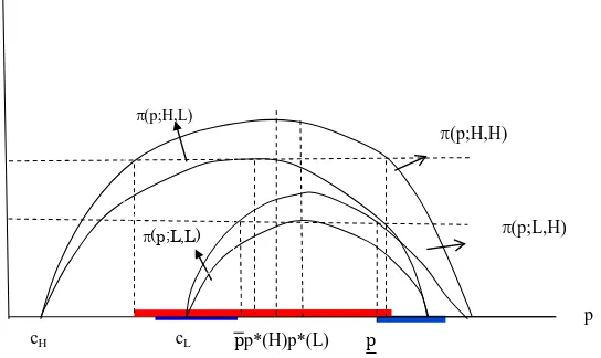
Hmust satisfy the incentive compatibility constraint of the low-quality monopolist. The region that satisfies the low-quality monopolist’s incentive compatibility constraint is illustrated in blue in Figure 1.
π(p;H,H) π(p;H,L)
π(p;L,L) π(p;L,H)
π
p cH cL
On the other hand, pH must also satisfy the incentive compatibility of the high-quality monopolist. A high-type monopolist choosing to send a costly signal must have no incentive to deviate to its optimal price when it is perceived to be a low-quality type. The region satisfying the high-quality type’s incentive compatibility constraint is illustrated in red in Figure 1.
Figure 1 shows that a high-quality type’s separating price, which satisfies both types’ incentive compatibility conditions, can be distorted either upward or downward. In other words, high-quality products can be signaled either by high or low prices However, if the cost-reducing investment sufficiently improves efficiency such that the resulting reduction in marginal cost exceeds the increase in demand, then we can show that, in this case, high quality can be signaled only by a low price.
Proposition 3 If cL−cH>∆≡H−L, then pH<pLin the unique separating equilibrium that passes the C-K Intuitive Criterion where pH<p∗(H).
The condition for the cost (cL−cH>∆)—which will be called separation condition (SC)—is crucial for signaling high quality via low price. This condition implies that the full-information price of anH-type monopolist is lower than that of anL-type monopolist. If the inequality of the condition is reversed, then high price signals high quality just as Schmalensee (1978) predicted.
The intuition behind this proposition goes as follows. If the optimal price for theH-type monopolist under complete information can be imitated by the L type, then the H-type’s equilibrium price must be distorted either upward or downward to signal its quality. Can the monopolist not charge a higher price to signal high quality? The answer is negative because more distortion is required in the upward direction so long asp∗(H)<p∗(L). Upward distortion is more costly forHtype. Therefore, if the monopolist charges a lower price than the upwardly distorted equilibrium price, then consumers should believe that the monopolist isHtype (for whom such a downward deviation is less costly) and notLtype; in fact, theLtype never gains by doing so. Hence,Htype will not stick to its equilibrium price. This overturns the equilibrium involving upward distortion. This also confirms the insight that the high-quality monopolist is more likely to gain by charging a lower price and thereby increasing sales because of its higher margin(cL>cH).
Our result that high quality can sometimes be signaled only by choosing a low price is not due to repeat purchases. So long as the true quality type is revealed (e.g., through word-of-mouth communication) right after the first period, assumptions about repeat purchases have no role in this model. A high-quality monopolist’s large sales volume achieved by offering a generously low introductory price in the first period does not, in our model, generate a large sales volume in the second period, which is determined independently of first-period sales volume. Therefore, the results in the Propositions above are not due to the Nelson effect, but simply due to the low production costs of the high-quality product, contrary to the precondition of the Schmalensee effect.
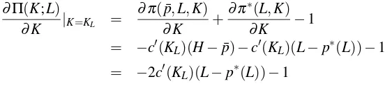
4.2 The First-Stage Investment Game
Letπ∗∗(r;K)be the r-type’s profit (from the viewpoint of the first period, i.e., revenue net of investment costsK) in the separating equilibrium in the pricing game under incomplete information. That is, π∗∗(r;K) =π(pr,K;r). Assuming that the separating equilibrium is played in the subsequent game, the monopolist’s investment decision will depend onπ∗∗(r;K). Denote the equilibrium investment of anr-type firm byKr.
We are mainly interested in the possibility of the investment-separating equilibrium in which KH>KL. In order to haveKH>KLin equilibrium, two conditions must be satisfied: incentive compatibility conditions for investment decisions, and incentive compatibility conditions for separating prices (or equivalently, the SC condition).
Lemma 2 In a separating equilibrium, KL=K∗(L).
First, it is easy to see that anyK6=K∗(L)cannot be an equilibrium investment level of the low-quality-type monopolist. IfKL6=K∗(L), then the low-quality-type monopolist would deviate toK∗(L) =arg maxΠ∗(K;L) =2(p∗(L)−c(K))(L−p∗(L))−K. SinceKis unobservable, any deviant choice ofKcannot affect consumer perceptions about quality. Some may wonder if a low-quality-type monopolist might benefit from deviating simultaneously from bothK∗(L)
and p∗(L). In the appendix, we will prove that payoff-improving deviations of this kind are not possible either.
SinceK cannot be used as a signal due to its unobservability, separation by signaling is possible only by using the first-period price (i.e., pH= p¯ and pL=p∗(L)). Therefore, the high-quality-type monopolist choosesKto satisfy
K=K¯H≡arg max
K Π
e(K)≡π(p¯,K,H) +π(p∗(c(K)),K;H)−K (7)
in a separating equilibrium.
Lemma 3 In a separating equilibrium, KH=K¯H.
Similarly, ifKH 6=K¯H, then the high-quality-type monopolist has an incentive to deviate to K=K¯Hwithout reputational losses (i.e., without risk of being perceived as a low-quality type). Again, in the Appendix, we provide a proof showing that the high-quality-type monopolist has no incentive to deviate from ¯KHand ¯psimultaneously.
It is clear thatKL<KHand, thus, it is possible to havecL≡c(KL)>c(KH)≡cH. Thus, if cLandcHsatisfy the SC condition, we have a separating equilibrium in which high quality is signaled by low price.
Proposition 4 There is a separating equilibriumin which KL<KH and pH <pL if the SC
condition holds.
the production cost. We may follow the spirit of Schmalensee (1978) more closely by assuming that the initial marginal costs of high-quality and low-quality types differ. Let the marginal cost be denoted byc(K;r)wherec(0;r) =c¯rand ¯cH>c¯L. We assume thatc(K;H)>c(K;L), c′(K;r)<0,c′′(K;r)>0,limK→0c′(K;r) =−∞and limK→∞c′(K;r) =0 for allKand for allr.
For example, we can assume thatc(K;r) =c¯r−s(K)wheres′(K)>0 ands′′(K)<0.
If the cost-saving investment is efficient enough to reverse the cost disadvantage ofHtype, then our result remains unaffected. If the cost-saving investment is so inefficient that it can hardly change the order ofc(KH;H)andc(KL;L), then it will not be an interesting case because Kplays little role in the model in that case. Neither case adds much to our analysis.
5 Conclusion and Caveats
In this paper, we reexamined the Schmalensee effect by considering a dynamic model of an experience good that incorporates the monopolist’s investment decision to reduce cost. We confirmed our insight that a high-quality monopolist does indeed have a stronger incentive to lower cost if consumers are not well informed about the quality of the product. This result may explain the phenomenon by which a high-quality firm would seem to expend more effort to reduce cost, as in the example in the Introduction about the Luna mobile phone.
We must admit, however, that our result is not very robust. We simply identified the third effect other than two already well known effects, Nelson effect and Schmalensee effect in explaining the pricing behavior of an experience good monopolist. If producing a high-quality product requires much costly technology, the incentive to lower the cost alone may not revert the original cost disadvantage, as discussed in Section 4. Also, the third effect is possible only if the monopolist engages in a process innovation reducing the marginal production cost, not in a quality-improving innovation. Readers may wonder if this is a relevant setup in reality. According to Whiteet al.(1988),9data seem to support the relevancy of our analysis at least weakly.
Appendix
Proof of Proposition 1: Total differentiation of equation (3) with respect to K andr yields dK∗/dr>0, sinceπKK<0 from the second order condition andπKr>0 fromD2>0. k
Proof of Proposition 2:(i) SinceD2>0,π(p,r)is increasing inrand so isΠ(p,K,r)for all pandK. Therefore, it is clear thatΠ∗(H)≡maxp,KΠ(p,K,H)>maxp,KΠ(p,K,Lr)≡Π∗(L). (ii) SinceK∗(H)>K∗(L)by Proposition 1, it must be the case thatπ(K∗(H),H)>π(K∗(L),L).
9 It states that in the sample of British small firms, 61 per cent of product innovators were process innovators as well,
Proof of Proposition 3: Note that p∗(H)<p∗(L) from the condition that cL−cH >∆. Figure 1 shows the set of separating equilibrium prices for theH-type firm. In the Figure, for an equilibrium pricepH<p¯, consider a slight deviation, pricep′=pH+ε<p¯, whereε >0. Then, a low-type firmX is worse off regardless of the posterior Belief, while a high-type firm X clearly benefits if it is perceived to be a high type. Since p′ is equilibrium -dominated to a low-type monopolist, we can apply the intuitive criterion to infer thatre=H. This leaves only the Riley outcome(pH,pL) = (p¯,p∗(L))involving the most efficient signaling as the equilibrium that passes C-K Intuitive Criterion. Now, for an equilibrium pricepH>p, consider a slight deviation p′′∈(p,pH). It also satisfies both (5) and (6). Therefore, it fails to pass
Proof of Lemma 2: It remains to show that a low-type monopolist has no incentive to imitate a high-type monopolist by choosing pHandK6=KL. Since only the price is observable, this deviation will lead tore=H. If he deviates fromKL, we have
We already know from Section 4.1 that(p,KH)cannot be a profitable deviation for the high type for anyp6=p¯. Now, let us consider a deviation(p,K)for p6=p¯andK6=KH. We use the most pessimistic belief: re =Lif p6=p¯is observed. Then, the high-type monopolist would chooseKsatisfying
Acknowledgements: This research was begun when Jeong-Yoo Kim was visiting POSTECH in 2015.
References
Bagwell, K., and M. Riordan (1991). High and Declining Prices Signal Product Quality. Eco-nomic Review81(1): 224–239.https://www.jstor.org/stable/2006797
Chenavaz, R. (2016). Better Product Quality May Lead to Lower Product Price.Journal of Theoretical Economics17(1): 1–22.
https://ideas.repec.org/a/bpj/bejtec/v17y2017i1p22n4.html
Cho, I., and D. Kreps (1987). Signalling Games and Stable Equilibria.Quarterly Journal of Economics102(2): 179–221.
Daughety, A., and J. Reinganum (1995). Product Safety: Liability, R&D, and Signaling. Eco-nomic Review85(5): 1187–1206.https://www.jstor.org/stable/2950983
Judd, K., and M. Riordan (1994). Price and Quality in a New Product Monopoly.Review of Economic Studies61(4): 773–789.https://www.jstor.org/stable/2297918
Kaya, A. (2013). Dynamics of Price and Advertising as Quality Signals: Anything Goes. Economics Bulletin33(3): 1556–1564.https://ideas.repec.org/a/ebl/ecbull/eb-13-00300.html
Kim, J.-Y. (2017). Pricing an Experience Composite Good as Coordinated Signals. The Manch-ester School 85(2): 163–182.
Lewis, T., and D. Sappington (1989). Countervailing Incentives in Agency Problems.Journal of Economic Theory49(2): 294–313.
http://www.sciencedirect.com/science/article/pii/0022053189900835
Maggi, G., and A. Rodriguez-Clare (1995). On Countervailing Incentives.Journal of Economic Theory66(1): 238–263.http://www.sciencedirect.com/science/article/pii/S002205318571040X
Milgrom, P., and J. Roberts (1986). Price and Advertising Signals of Product Quality.Journal of Political Economy94(4): 796–821.https://www.jstor.org/stable/1833203
Nelson, P. (1970). Information and Consumer Behavior.Journal of Political Economy78(2): 311–329.https://www.jstor.org/stable/1830691
Nelson, P. (1974). Advertising as Information.Journal of Political Economy81(4): 729–754. https://www.jstor.org/stable/1837143
Schmalensee, R. (1978). A Model of Advertising and Product Quality.Journal of Political Economy86(3): 485–503.https://www.jstor.org/stable/1833164
White, M., H.J. Braczyk, A. Ghobadian, and J. Niebuhr (1988). Small Firms’ Innovation: Why Regions Differ. Policy Studies Institute.
Wolinsky, A. (1983). Price as Signals of Product Quality.Review of Economic Studies50(4): 647–658.https://www.jstor.org/stable/2297767
Please note:
You are most sincerely encouraged to participate in the open assessment of this article. You can do so by posting comments.
Please go to:
http://dx.doi.org/10.5018/economics-ejournal.ja.2017-5
The Editor