Full Terms & Conditions of access and use can be found at
http://www.tandfonline.com/action/journalInformation?journalCode=cbie20
Bulletin of Indonesian Economic Studies
ISSN: 0007-4918 (Print) 1472-7234 (Online) Journal homepage: http://www.tandfonline.com/loi/cbie20
Indonesia's Non-Oil Export Performance During
the Economic Crisis: Distinguishing Price Trends
from Quantity Trends
L. Peter Rosner
To cite this article:
L. Peter Rosner (2000) Indonesia's Non-Oil Export Performance During
the Economic Crisis: Distinguishing Price Trends from Quantity Trends, Bulletin of Indonesian
Economic Studies, 36:2, 61-95, DOI: 10.1080/00074910012331338893
To link to this article:
http://dx.doi.org/10.1080/00074910012331338893
Published online: 18 Aug 2006.
Submit your article to this journal
Article views: 87
View related articles
INDONESIA’S NON-OIL EXPORT
PERFORMANCE DURING THE ECONOMIC
CRISIS: DISTINGUISHING PRICE TRENDS
FROM QUANTITY TRENDS
L. Peter Rosner*
Harvard Institute for International Development (HIID)
Despite an enormous currency depreciation, the growth rate of Indonesia’s non-oil exports, measured in dollars, did not accelerate during the first two years of the Asian crisis. In fact, during the second year of the crisis non-oil export value dropped sharply. This paper demonstrates that the main reason for the decline in the dollar value of non-oil exports was a collapse of export prices. Non-oil export dollar prices fell 26% between the second quarter of 1997 and the second quarter of 1999. Measured at constant prices, non-oil exports grew 24% and manufactured exports 31% during this period. Non-oil import prices fell by roughly the same amount as non-oil export prices during the crisis, with little change in the non-oil terms of trade. The decline in the price of traded goods significantly reduced the magnitude of the real exchange rate depreciation experienced by Indonesia.
INTRODUCTION
rose from 0% in 1985 to 11% in 1986, 31% in 1987 and 34% in 1988. Past econometric research also found a strong link between the real exchange rate and export growth in Indonesia. For example, using quarterly data from 1985–94, Radelet (1996) estimated a price elasticity of supply for non-oil exports of 0.778, implying that a 10% depreciation of the real exchange rate would lead to a 7.78% rise in non-oil exports. Before the onset of the East Asian currency crisis, therefore, Indonesia’s experience with exchange rate depreciations had been relatively straightforward: large depreciations (or devaluations) were followed by large increases in the growth rate of non-oil export value, sustained over several years.
Indonesia’s experience during the recent crisis has been very different. Despite a massive depreciation of the currency, non-oil export value growth fell from +10% in 1997 to –2% in 1998 and to –6% in 1999. Far from stimulating export growth, the 1997–98 depreciation appeared to result in an unprecedented collapse of non-oil exports.
Several explanations for this surprising development have been popularised. The most common is that the collapse of the domestic banking system made trade finance unavailable to exporters. According to this explanation, export firms were unable to finance imports of raw materials and components, and did not have access to working capital for day-to-day operations, preventing them from taking advantage of the depreciation (Pardede 1999; FEER, 14/1/99; JP, 19/10/99). Reduced demand in importing countries, particularly in East Asia, has also been blamed for the export slowdown. A third argument sometimes heard is that Indonesia’s export industries are too dependent on imported inputs. With the collapse of the rupiah, according to proponents of this view, imported inputs have become too expensive. Policy makers have therefore drawn the conclusion that import-dependent export industries are unreliable and that future export promotion efforts should focus on industries that process domestic raw materials.1 A fourth explanation is
that social and political instability in Indonesia in 1998 and 1999 caused international buyers of manufactured products to shift orders to other countries, particularly in the wake of the May 1998 riots in Jakarta.
steadily since the onset of the regional economic crisis. For example, the World Bank’s index of non-energy commodity prices for low and middle income developing countries declined from 126.0 in the second quarter of 1997 to 87.8 in the second quarter of 1999 and to 85.8 by July 1999 (World Bank, Global Commodity Markets, table A1, various issues). This represents a decline of 32% over a two-year period.2
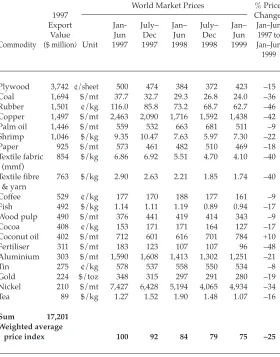
Prices for Indonesia’s major non-oil export commodities have followed a similar trend. As can be seen in table 1, prices for 20 of Indonesia’s most important non-oil export commodities, comprising 42% of non-oil export value in 1997, fell by an average of 25% between the first half of 1997 and the first half of 1999. World market prices for many other items such as garments and footwear also fell. One of the prime reasons for the poor performance of Indonesia’s non-oil exports over the past two years is this sharp drop in export prices. Any analysis of recent export performance must therefore distinguish between price movements and quantity movements. There is no reason to expect, and economic theory does not postulate, that export value will rise following a currency depreciation—only a rise in export quantity should be expected.3
Some observers have recognised that Indonesian export prices declined during the crisis, causing a divergence between trends in export value and export volume. For example, James (2000) notes that if Indonesian non-oil export values are deflated using an import price index for the United States, non-oil exports in constant dollar prices rose 1.58% in 1998, although they fell by 2% when measured in current dollars. However, the composition of US imports and Indonesian non-oil exports is quite different, so the US import price index is at best a rough proxy for export prices faced by Indonesia.
Unfortunately, a satisfactory aggregate measure of either non-oil export volume or export price does not yet exist for Indonesia. The central statistics agency (BPS) publishes quantity data in kilograms for individual export items, but does not publish an aggregate volume index. It does publish a rupiah-based wholesale price index (WPI) for exports, but the non-oil component of the index includes only 43 items, of which less than 20 are manufactured products, and the index is therefore not representative of overall non-oil exports (BPS 2000).4 The International
Monetary Fund (IMF) publishes a monthly export volume index, but the IMF’s index is an unweighted average (or simple sum) of export tonnage.5
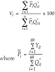
This paper addresses the lack of an appropriate measure of non-oil export volume by using unit values (export value in dollars divided by export quantity in kilograms) to construct an aggregate measure of monthly non-oil exports at constant prices. If we hold prices fixed, movements in export value can only be due to quantity changes. This is equivalent to measuring export volume by constructing a weighted average of export quantity indices, with the weights being the value share of each item in total non-oil exports. Once a volume index has been constructed, an implicit export price index can be derived simply by dividing export value by export volume.
To measure non-oil exports at constant prices, the data are first cleaned for extreme quantity outliers, and a base time period is selected for deriving constant export prices from export unit values. The analysis is conducted at the Harmonised System (HS) nine-digit level so as to minimise aggregation problems inherent in the use of unit values as a measure of export prices. After describing the methodology, we present findings for non-oil exports as a whole and for selected subsectors over the 69-month period April 1994 through December 1999.
MEASURING NON-OIL EXPORT VOLUME: METHODOLOGY
Our measure of non-oil export volume can be expressed as follows:
This is equivalent to measuring non-oil export volume as a weighted average of quantity indices for each item, i.e.:
TABLE 1 World Market Prices for Indonesia’s Major Non-oil Export Commodities
World Market Prices % Price
1997 Change
Export Jan- July– Jan– July– Jan– Jan–Jun
Value Jun Dec Jun Dec Jun 1997 to
Commodity ($ million) Unit 1997 1997 1998 1998 1999 Jan–Jun 1999
Plywood 3,742 ¢/sheet 500 474 384 372 423 –15 Coal 1,694 $/mt 37.7 32.7 29.3 26.8 24.0 –36 Rubber 1,501 ¢/kg 116.0 85.8 73.2 68.7 62.7 –46 Copper 1,497 $/mt 2,463 2,090 1,716 1,592 1,438 –42
Palm oil 1,446 $/mt 559 532 663 681 511 –9
Shrimp 1,046 $/kg 9.35 10.47 7.63 5.97 7.30 –22
Paper 925 $/mt 573 461 482 510 469 –18
Textile fabric 854 $/kg 6.86 6.92 5.51 4.70 4.10 –40 (mmf)
Textile fibre 763 $/kg 2.90 2.63 2.21 1.85 1.74 –40 & yarn
Coffee 529 ¢/kg 177 170 188 177 161 –9
Fish 492 $/kg 1.14 1.11 1.19 0.89 0.94 –17
Wood pulp 490 $/mt 376 441 419 414 343 –9
Cocoa 408 ¢/kg 153 171 171 164 127 –17
Coconut oil 402 $/mt 712 601 616 701 784 +10 Fertiliser 311 $/mt 183 123 107 107 96 –48 Aluminium 303 $/mt 1,590 1,608 1,413 1,302 1,251 –21
Tin 275 ¢/kg 578 537 558 550 534 –8
Gold 224 $/toz 348 315 297 291 280 –19
Nickel 210 $/mt 7,427 6,428 5,194 4,065 4,934 –34
Tea 89 $/kg 1.27 1.52 1.90 1.48 1.07 –16
Sum 17,201
Weighted average
price index 100 92 84 79 75 –25
where wi is the value share for item i in the base time period, or:
Export prices (the Pis) are derived from export unit values, measured
as export value divided by export quantity. A weakness in using unit values to measure export prices is that changes in unit values can reflect either true price changes or a change in the mix of items exported under a given export line. For relatively homogeneous items such as minerals and agricultural products it is reasonable to assume that a given export line will track the same item over time. But for manufactured goods the mix of items in a single export line frequently changes over time. For example, an export line identified as ‘colour TV sets’ might contain 14-inch sets one month and 19-inch sets the next. Moreover, export quantity is generally measured in kilograms, and kilograms are clearly a crude measure of quantity for manufactured goods.6
To avoid the aggregation problem inherent in the use of unit values, it would be necessary to have direct price observations for individual export items. Given the heterogeneity of manufactured exports this is not possible. A typical garment export firm, for example, frequently exports 100 or more different types of garments. Even a narrowly defined item such as ‘men’s cotton dress shirts’ could contain items of vastly different quality. In fact, for brand name garments each order is unique, so that even with the most detailed data imaginable it would not be possible to construct a perfect time series of the price of ‘men’s cotton dress shirts’. Given this inherent measurement problem and the limitations of Indonesian trade data, any measure of export volume or price that is representative of overall exports must rely on unit values.
the HS nine-digit level, the measure of non-oil export volume presented below is less influenced by aggregation bias than other measures of non-oil export volume that use a higher level of aggregation.
Data Source
The data for this analysis are BPS monthly export data for the period April 1994 through December 1999. BPS trade data record exports by both HS and SITC (Standard International Trade Classification) nine-digit codes. Since exporters record only the HS code on the export declaration form they submit to customs, and since the mapping from HS codes to SITC codes is subject to error, the HS codes are more reliable. The two key variables available in the monthly data for each HS line are the value of exports in dollars and the quantity of exports measured in kilograms.
Cleaning the Data
Unfortunately, BPS export data contain significant errors, particularly in the quantity variable. For example, exports of gold (HS line 7108.12.100) in January 1998 were recorded as 831.3 tonnes. This was more than 100 times greater than any previous or subsequent monthly quantity of gold exports, and implied that Indonesia sold gold for $71 per tonne in January 1998, as against a minimum price of more than $5,000 for any other month. Similarly, exports of unbleached cotton fabric (HS line 5208.12.900) were recorded at 102,999 tonnes in December 1998, exceeding any previous or subsequent quantity by a factor of 48 and implying that cotton fabric was sold for 12¢ per kilogram in December 1998 as against a minimum price of $3.24 for any other month.
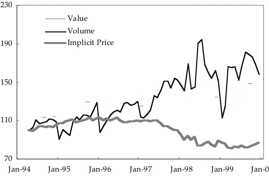
Because of these large data errors, any quantity index constructed from uncleaned data produces unreliable results. This can be seen in figure 1, which applies equation (1) to raw BPS export data. The index is highly volatile, particularly in 1997 and 1998, with month-to-month changes in excess of 20% that bear little relationship to changes in export value. The uncleaned quantity index is particularly volatile in mid 1998, with volume growth of 57% recorded between May and July, followed by a decline of 22% in August.
To respond to the data error problem, we developed a simple data cleaning algorithm. Our algorithm assumes that the export values for each HS line in each month are correct and that all problems lie in the quantity
variable.7 Any excessive change in the unit value (value divided by
unit value in the previous non-zero month is the correct unit value, and we define a new ‘cleaned’ quantity by dividing the current month’s unit value by the previous month’s unit value. In other words, our cleaning algorithm can be expressed as follows:
if (Pit/Pit–1) > x or (Pit/Pit–1) < (1/x) then Qit* = Yit/Pit–1 and Pit = Pit–1 (4)
where x is the cleaning factor, Yit is the dollar value of item i exported in time t, Pit–1 is the unit value of item i in the previous (non-zero) time period and Qit* is the cleaned quantity. The cleaned Qit* are then used to
construct new unit values for the calculation of fixed base-period export prices, and are also used in equation (1) above.8
The decision about what constitutes an ‘excessive’ month-to-month change in the unit value for a particular export item is subjective. We decided that anything greater than a fivefold change was definitely excessive and anything less than a twofold change was within the bounds of the possible. We then experimented with various cleaning factors (x
values in equation (4)). The results for x = 2, x = 3, x = 4 and x = 5 are discussed in more detail in the appendix.
Choice of a Base Time Period for Calculating Constant Prices
The choice of time period for constructing constant prices is not clearly determined by economic theory, and yet can have an impact on the resulting measure of export volume. Measuring 1994–99 non-oil exports at constant 1994 prices produces different results from those obtained using constant 1996 prices or constant 1998 prices. In broad terms, the choice is between using current prices and projecting them back or using past prices and projecting them forward—the difference between a Paasche and a Laspeyres index. Ideally the difference between these two indices would not be large, but in practice it turns out to be significant. This is because the fixed prices are essentially weights, as was shown in equation (2) above, and the weights change significantly over time as export value shares change.
particular HS line in a single month could have a major impact on the volume index if data from that month alone were used to create the fixed price for each item, but if the fixed prices for each item are calculated from many months of data the sensitivity of the results to outliers is reduced. This consideration argues for using a period of at least 12 months, and perhaps longer, for calculating the fixed price for each item.
Experiments with the data indicated that even calculating the fixed prices from annual data produced significantly different results depending on which year was chosen. Measuring exports at constant 1996 prices, for example, resulted in higher 1998 volume growth than measuring them at constant 1997 prices, and using constant 1998 prices produced the lowest measure of export volume growth in 1998. These differences are presented and discussed in the appendix. To avoid having to select a single year’s export prices as the ‘correct’ prices, it was decided to use the average price for each item over the entire 69-month time period for which data were available.
FIGURE 1 Non-oil Export Value, Volume and Price before Cleaninga (monthly index April 1994 to December 1999; April 1994 = 100)
aThe export volume index uses constant average 1994–99 prices. The export
quan-tity for gold in January 1998 has been cleaned. If the published number of 831 tonnes is used, the volume index rises to more than 500 in January 1998.
70 110 150 190 230
Jan-94 Jan-95 Jan-96 Jan-97 Jan-98 Jan-99 Jan-00 Value
The methodology ultimately selected for measuring non-oil export volume therefore uses a modified version of equation (1), which can be expressed as:
FINDINGS: EXPORT VOLUME AND PRICES BEFORE AND DURING THE CRISIS
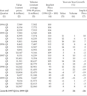
Figure 2 presents the results of applying the methodology described above to monthly BPS export data over the period April 1994 to December 1999. Non-oil export volume is measured at constant average 1994–99 prices with a cleaning factor of x = 3, meaning that any month-to-month change in the unit value within a particular HS line that exceeds a factor of 3 is assumed to reflect a mistake in the quantity data, and a new quantity variable is then created using the previous month’s unit value and the current month’s value. The cleaned volume index is less volatile than the uncleaned index shown in figure 1, and bears a stronger resemblance to the non-oil export value index.
Figure 2 shows that the average price of non-oil exports rose in 1994 and 1995 and then fell very slightly from early 1996 through mid 1997. In mid 1997 non-oil export prices began a steep decline that continued through early 1999. By the second quarter of 1999 they had dropped by 26% relative to the same period two years earlier.
As can be seen in the sixth column of the table, export volume growth was lower than export value growth from 1995 through the first half of 1996, and very slightly above it from mid 1996 until mid 1997, but in the third quarter of 1997 export volume growth accelerated sharply. Year-on-year volume growth peaked at 32% in the first quarter of 1998 and then declined during the second and third quarters of 1998, but remained well above historical levels. By contrast, export value growth turned
TABLE 2 Quarterly Non-oil Exports: Value, Volume and Price, 1994–1999
Volume Year-on-Year Growth Value (constant Implicit (%) (current average Price
Year and prices; 1994–99 prices; Index Implicit Quarter $ million) $ million) (1994 Q2 = 100) Value Volume Price
(1) (2) (3) (4) (5) (6) (7)
1994 Q2 7,589 7,502 100 Q3 8,154 7,772 104 Q4 8,339 7,919 104 1995 Q1 7,583 6,945 108
Q2 8,395 7,574 110 11 1 10 Q3 9,165 8,235 110 12 6 6 Q4 9,811 8,684 112 18 10 7 1996 Q1 8,462 7,487 112 12 8 4 Q2 9,593 8,507 111 14 12 2 Q3 9,891 8,993 109 8 9 –1 Q4 10,147 9,166 109 3 6 –2 1997 Q1 9,151 8,239 110 8 10 –2 Q2 10,411 9,354 110 9 10 –1 Q3 11,311 10,637 105 14 18 –3 Q4 10,997 10,779 101 8 18 –8 1998 Q1 10,242 10,901 93 12 32 –15 Q2 10,272 11,455 89 –1 22 –19 Q3 10,804 12,470 86 –4 17 –19 Q4 9,657 11,188 85 –12 4 –15 1999 Q1 8,296 9,687 85 –19 –11 –9 Q2 9,634 11,573 82 –6 1 –7 Q3 10,555 12,613 83 –2 1 –3 Q4 10,387 12,060 85 8 8 0
Growth 1997 Q2 to 1999 Q2 –7 24 –26
negative after the first quarter of 1998. In the final quarter of 1998 volume growth slowed and then became negative in the first quarter of 1999, but it remained much higher than value growth. In the second quarter of 1999 volume growth recovered to plus 1%, and reached 8% by the fourth quarter, even though value growth remained negative through the third quarter.9
Figure 2 shows that most of the growth in non-oil export volume took place during the first year of the economic crisis. Although volume was still 17% higher during the third quarter of 1998 than it had been a year earlier, on a month-to-month basis it began declining in August 1998 and continued to drop sharply through early 1999. During January and February 1999, non-oil export volume fell to its lowest level in three years. It recovered in March 1999 and continued to grow through August 1999, but during the period March–August 1999 it was still 2% lower than it had been during the same period in 1998.
The apparent slowdown in the growth of non-oil export volume after mid 1998 may have been caused partly by the civil unrest that accompanied the political transition occurring at that time. It may also have been due to the fact that export volumes had reached a very high level in the first half of 1998, with much of the growth caused by one-off export activities that were not sustainable. During the first half of 1998
FIGURE 2 Non-oil Export Value, Volume and Price, Using Cleaned Quantity Data (monthly index April 1994 to December 1999; April 1994 = 100)
70 110 150 190 230
Jan-94 Jan-95 Jan-96 Jan-97 Jan-98 Jan-99 Jan-00
the value of the rupiah dropped at an unprecedented rate, falling from Rp 4,650/$ at the end of 1997 to more than Rp 15,000/$ by mid 1998. The magnitude and speed of the depreciation created opportunities for windfall profits from trade, as local prices did not always adjust up as rapidly as the rupiah was falling. A large quantity of merchandise appears to have been exported during an ‘arbitrage window’ in the first half of 1998, as traders took advantage of the speed of the rupiah depreciation to purchase existing stocks of goods in Indonesia and ship them abroad. Toward the end of the third quarter of 1998, as the rupiah began to strengthen and local prices caught up with international prices, this window may have begun to close, contributing to a decline in these ‘one-off’ exports.
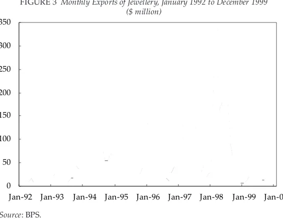
Evidence of ‘one-off’ export activity can be seen in the pattern of jewellery exports. Between January and March 1998, monthly jewellery exports rose from less than $50 million to a record level of $337 million. During the first half of 1998 the value of jewellery exports reached $1.3 billion, three times greater than a year earlier, and jewellery accounted for more than one-third of the growth of non-oil export value over this period. In August 1998 jewellery exports suddenly collapsed and by the end of 1998 were below pre-crisis levels. The pattern seen in figure 3 strongly suggests a depreciation-induced boom motivated by pure trading opportunities, followed by a bust as the arbitrage window closed.10 A similar pattern can be seen in wood pulp exports, which grew
enormously during the period January–July 1998 and then dropped suddenly toward the end of 1998. With jewellery and wood pulp excluded, non-oil export volume grew by 9% during the second quarter of 1999 relative to the same period in the previous year.
Toward the latter part of 1999 export prices began to recover (figure 2). The monthly index of non-oil export prices, calculated as the ratio of export value to export volume, increased from 82 in September 1999 to 87 in December 1999. This upturn coincided with a recovery in world market prices for commodities as recorded in international data sources. For example, the World Bank’s ‘Pink Sheet’ series shows that prices of copper, nickel, aluminium, gold, steel and wood pulp all turned up strongly in the second half of 1999, and plywood prices were 32% higher in the fourth quarter of 1999 than they had been in the third quarter of 1998.11 The stabilisation and partial recovery of export prices in late
1999 allowed the relatively strong growth of non-oil export volume during the crisis to show up as higher dollar revenue, and was probably the main factor behind the 29.6% year-on-year rise in non-oil export value reported during the first quarter of 2000.
THE SOURCES OF NON-OIL EXPORT GROWTH: SECTORAL ANALYSIS
The preceding analysis has shown that non-oil export volume continued to grow strongly during the economic crisis and that the drop in export revenue, measured in dollars, was caused mainly by declining export
0 50 100 150 200 250 300 350
Jan-92 Jan-93 Jan-94 Jan-95 Jan-96 Jan-97 Jan-98 Jan-99 Jan-00 FIGURE 3 Monthly Exports of Jewellery, January 1992 to December 1999
($ million)
prices. The strong growth of non-oil export volume was interpreted as an indication that trade finance problems did not prevent exporters from taking advantage of the enormous increase in competitiveness caused by the depreciation of the rupiah.
However, not all of Indonesia’s non-oil exports require significant quantities of imported inputs. Almost one-half of non-oil exports consist of primary commodities and semi-processed resource-based products with low import content, such as coal, rubber, palm oil and plywood. Since exporters of these products generally do not need to open letters of credit for imported inputs before each export shipment, it is possible that even a very serious trade finance problem would not greatly affect them. If the growth of export volume during the crisis has been driven mainly by exports of primary commodities and semi-processed products, and if manufactured exports have stagnated or declined, this would suggest that trade finance problems might be having more of an impact than would be assumed from the aggregate export volume data alone. It is therefore important to look at the source of non-oil export volume growth by sector.
To investigate the source of non-oil export volume growth, non-oil exports were divided into four broad categories: (1) agriculture and related semi-processed products; (2) forestry products (including plywood, pulp, paper and semi-processed forestry products); (3) mining and mineral products; and (4) manufactured goods.12 The results of this
analysis are shown in table 3. As can be seen in the last row of the table, manufactured exports did better during the crisis than any of the other three categories, in both value and volume terms. Measured in dollars, manufacturing was the only category to experience growth between the second quarter of 1997 and the second quarter of 1999. Export value for the other three categories contracted sharply. Measured by volume, all four categories experienced growth over this two-year period, but manufacturing experienced by far the strongest growth.
L
. Pet
er Ro
sner
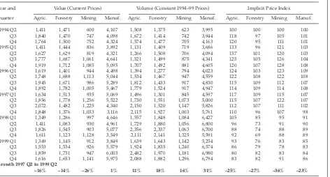
Year and Value (Current Prices) Volume (Constant 1994–99 Prices) Implicit Price Index
Quarter Agric. Forestry Mining Manuf. Agric. Forestry Mining Manuf. Agric. Forestry Mining Manuf.
1994 Q2 1,411 1,471 600 4,107 1,508 1,375 623 3,995 100 100 100 100
Q3 1,840 1,470 747 4,098 1,672 1,414 742 3,944 118 97 105 101
Q4 1,764 1,500 752 4,324 1,574 1,477 705 4,163 120 95 111 101
1995 Q1 1,411 1,444 836 3,892 1,131 1,409 719 3,686 133 96 121 103
Q2 1,627 1,629 819 4,321 1,266 1,508 706 4,094 137 101 120 103
Q3 1,777 1,687 1,061 4,641 1,521 1,499 875 4,341 125 105 126 104
Q4 1,919 1,712 1,085 5,095 1,707 1,492 881 4,605 120 107 128 108
1996 Q1 1,619 1,401 944 4,498 1,394 1,277 794 4,023 124 103 123 109
Q2 1,748 1,688 1,113 5,044 1,534 1,467 947 4,559 122 108 122 108
Q3 1,945 1,671 986 5,289 1,812 1,433 917 4,830 115 109 112 107
Q4 1,892 1,782 1,005 5,467 1,779 1,524 917 4,947 114 109 114 108
1997 Q1 1,634 1,513 935 5,069 1,496 1,301 845 4,597 117 109 115 107
Q2 1,856 1,778 1,256 5,522 1,730 1,551 1,073 5,000 115 107 122 107
Q3 2,072 1,482 1,225 4,340 2,150 1,520 1,147 5,826 112 107 111 102
Q4 1,848 1,376 1,033 3,116 2,115 1,927 1,003 5,761 110 96 107 98
1998 Q1 1,349 1,286 997 4,646 1,557 1,848 1,084 6,427 105 85 95 91
Q2 1,411 1,083 930 4,961 1,729 1,880 1,056 6,800 96 73 91 90
Q3 1,826 1,545 903 5,077 2,356 2,337 1,063 6,700 88 74 88 89
Q4 1,611 1,123 1,128 3,549 2,111 2,141 1,325 5,591 92 69 88 89
1999 Q1 1,349 1,145 912 3,849 1,639 1,643 1,142 5,254 93 76 83 85
Q2 1,553 1,534 926 5,579 1,924 1,835 1,240 6,574 86 79 78 83
Q3 1,859 1,731 947 6,003 2,482 1,970 1,181 6,980 80 82 83 84
Q4 1,616 1,653 1,141 5,975 2,088 1,882 1,296 6,794 83 82 91 86
Growth 1997 Q2 to 1999 Q2
–16% –14% –26% 1% 11% 18% 16% 31% –25% –27% –36% –23%
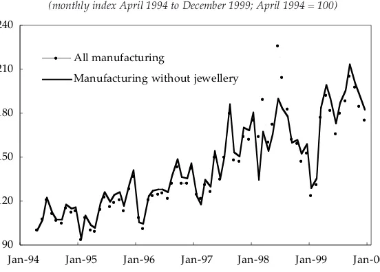
Figure 4 also shows that exports of manufactured goods declined sharply during the second half of 1998. This decline began roughly three months after the May 1998 riots. Many manufactured export products, such as garments and footwear, typically have a lag of about three months between the time orders are placed and the time merchandise is shipped out of the country. The timing of the sharp drop in manufactured exports in the second half of 1998 is consistent with the assertion that international buyers shifted orders to other countries in response to the May 1998 riots and the continued political instability in Indonesia in 1998. Interviews with textile, garment and footwear manufacturers conducted by the author in the second half of 1998 confirmed that many companies suffered a severe cutback in orders following the riots. However, the strong recovery of manufactured exports after February 1999 indicates that this impact was largely temporary.
Looking at export price trends by sector, table 3 shows that all four non-oil export sectors suffered from sharply falling dollar prices in 1997– 99. Prices for manufactured products declined the least, dropping by 23% between the second quarter of 1997 and the second quarter of 1999, but
FIGURE 4 Export Volume of Manufactured Goods Excluding Jewellery (monthly index April 1994 to December 1999; April 1994 = 100)
Source: Calculated from BPS trade data. 90
120 150 180 210 240
Jan-94 Jan-95 Jan-96 Jan-97 Jan-98 Jan-99 Jan-00
All manufacturing
this decline was only slightly less than the 25% drop in the average price of agricultural exports. Average export prices fell by 27% for forestry products and by 36% for mining and mineral products.
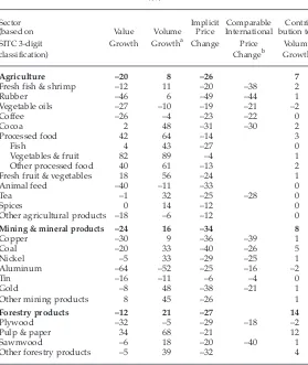
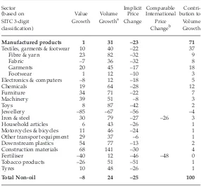
A more detailed analysis of the source of non-oil export growth during the economic crisis is provided in table 4, which disaggregates non-oil exports into 45 items and subsectors. For each item or subsector, the table
TABLE 4 Non-oil Exports by Sector: Value Growth, Volume Growth and Price Change, April–July 1997 to April–July 1999
(%)
Sector Implicit Comparable Contri-(based on Value Volume Price International bution to SITC 3-digit Growth Growtha Change Price Volume classification) Changeb Growth
Agriculture –20 8 –26 7
Fresh fish & shrimp –12 11 –20 –38 2
Rubber –46 6 –49 –44 1
Vegetable oils –27 –10 –19 –21 –2
Coffee –26 –4 –23 –22 0
Cocoa 2 48 –31 –30 2
Processed food 42 64 –14 3
Fish 4 43 –27 0
Vegetables & fruit 82 89 –4 1
Other processed food 40 61 –13 2
Fresh fruit & vegetables 18 56 –24 1
Animal feed –40 –11 –33 0
Tea –1 32 –25 –28 0
Spices 0 14 –12 0
Other agricultural products –18 –6 –12 0
Mining & mineral products –24 16 –34 8
Copper –30 9 –36 –39 1
Coal –20 33 –40 –26 5
Nickel –5 33 –29 –25 1
Aluminum –64 –52 –25 –16 –2
Tin –16 –11 –6 –4 0
Gold –8 48 –38 –21 1
Other mining products 8 45 –26 1
Forestry products –12 21 –27 14
Plywood –32 –5 –29 –18 –2
Pulp & paper 34 68 –21 12
Sawnwood –6 18 –20 –40 1
shows the growth rate of export value and volume and the change in the implicit export price between the four-month period April–July 1997 and the same period in 1999.13 The table also shows price changes for similar
items from international data sources, where available.
Table 4 shows that average export prices declined for every one of the 45 items and subsectors over this two-year period, with the largest price decline in the mining sector and the smallest in the manufacturing
TABLE 4 (continued) Non-oil Exports by Sector: Value Growth, Volume Growth and Price Change, April–July 1997 to April–July 1999
(%)
Sector Implicit Comparable Contri-(based on Value Volume Price International bution to SITC 3-digit Growth Growtha Change Price Volume classification) Changeb Growth
Manufactured products 1 31 –23 71
Textiles, garments & footwear 10 40 –22 37
Fibre & yarn 23 82 –32 9
Fabric –7 36 –32 8
Garments 20 45 –17 18
Footwear 1 12 –10 3
Electronics & computers –8 12 –18 5
Chemicals 19 64 –28 12
Furniture 34 71 –22 7
Machinery 39 51 –8 3
Toys 8 87 –42 2
Jewellery –85 –67 –56 –4
Iron & steel 30 79 –27 –26 3
Household articles 6 43 –26 1
Motorcycles & bicycles 11 46 –24 1
Other transport equipment 29 37 –6 1
Downstream plastics 54 77 –13 2
Construction materials 68 141 –30 4
Fertiliser –40 12 –46 –48 0
Tobacco products –26 51 –51 1
Tyres 10 48 –26 1
Total Non-oil –8 24 –25 100
aCalculated using constant average unit values over the period January 1996 to
September 1999.
sector. The price changes calculated from Indonesian trade data are generally similar to price changes reported in international publications, although for some items Indonesian export prices changed more, and for others less, than reported world market prices.
The last column of table 4 shows the contribution of each item to non-oil export volume growth between April–July 1997 and April–July 1999. Manufacturing accounted for 71% of volume growth over this period, even though it represented less than 55% of non-oil export volume (and value) at the start of the period. The item that made the greatest contribution was garments, which accounted for 18% of all non-oil export volume growth over this period. Chemicals and pulp and paper each accounted for 12% of volume growth, fibre and yarn for 9%, fabric for 8%, and furniture for 7%, while coal and electronics each accounted for 5% of volume growth. The volume growth data indicate that export sectors that are heavily dependent on imported inputs, such as garments, textiles, chemicals, toys, and transport equipment, experienced rapid export volume growth during the economic crisis.14 On the other hand,
so did some sectors that are dependent on domestic natural resources, such as pulp and paper, furniture, processed food and coal.
COMPARISON WITH OTHER REGIONAL ECONOMIES
Indonesia’s experience with sharply falling export prices during the regional economic crisis was apparently not unique. Data from Thailand and Korea indicate that both of these countries also experienced a sharp decline in export prices between 1997 and 1999. Export price indices for Indonesia, Korea and Thailand are shown in figure 5 (re-based so that July 1997 equals 100 to facilitate comparison). As can be seen in the figure, export prices declined by at least 20% in all three countries during the crisis. Relative to July 1997 Indonesia suffered the sharpest decline, but export prices for Korea had been declining since mid 1995, and by mid 1999 had fallen more than 30% in four years. Export prices for Thailand began to decline in early 1997 and by late 1999 had fallen by as much as Indonesian non-oil export prices.
Although their export prices declined to a similar extent, other regional economies did not suffer as drastic a fall in export values as did Indonesia. During the first year of the crisis Indonesia’s non-oil exports (measured in dollars) grew considerably faster than total dollar exports from Korea or Thailand. However, during the second year Indonesia’s non-oil export value declined by 12.2%, whereas total Korean export value declined by 2.4% and total Thai export value by 3.4% (table 5). Moreover, Korean and Thai export values recovered strongly in 1999 and had surpassed pre-crisis levels by the end of the year, whereas Indonesian non-oil export values remained well below pre-crisis levels in 1999. This suggests that Indonesian exports suffered from more than just a drop in prices, at least during the second year of the crisis. It is possible that the slowdown in non-oil export volume growth between August 1998 and February 1999 was a very delayed reaction to the trade finance problem that started in late 1997. However, given that the slowdown began three
FIGURE 5 Export Price Indices, Indonesia, Korea and Thailand (July 1997 = 100)
Sources: Indonesia: calculated from BPS export data using HS nine-digit unit values. Korea: IMF, International Financial Statistics.
Thailand: Bank of Thailand homepage (www.bot.or.th/bothomepage/ databank).
70 80 90 100 110 120
Jan-94 Jan-95 Jan-96 Jan-97 Jan-98 Jan-99 Jan-00
Thailand (export unit value)
Korea (export price)
months after the May 1998 riots, and given that non-oil export volume recovered strongly in mid 1999 even though trade finance problems continued, it seems likely that the August 1998 – February 1999 drop in non-oil exports was due mainly to the impact of social and political instability on international demand for Indonesian manufactured products.
TERMS OF TRADE AND THE REAL EXCHANGE RATE
The finding that non-oil export prices declined by around 26% in dollar terms during the crisis suggests a massive deterioration in Indonesia’s terms of trade. This raises the possibility that a major correction in the exchange rate might have been required to maintain Indonesia’s balance of payments even in the absence of the banking crisis, political instability and the numerous other problems that the country faced from mid 1997 on. However, the terms of trade depend on both export and import prices. Information on import price trends is therefore needed before any conclusion can be drawn about changes in the terms of trade.
TABLE 5 Annual Growth of Export Value, Indonesia, Thailand and Korea (%)
Perioda Year-on-Year Export Growth
Indonesia (non-oil) Thailand Korea
1994/95 to 1995/96 13.8 9.2 15.4
1995/96 to 1996/97 7.8 –2.0 1.0
——————————————————— start of crisis ——————————
1996/97 to 1997/98 7.3 2.0 3.0
1997/98 to 1998/99 –12.2 –3.4 –2.4
aEach time period starts in August so as to coincide with the floating of the
Indo-nesian rupiah. Thus ‘1994/95’ refers to the 12-month period August 1994 to July 1995. The first two rows are therefore pre-crisis growth rates.
The methodology discussed above for calculating export volume and an implicit export price index can easily be extended to import data. One practical problem with Indonesian import data is that the national statistics agency does not report imports into export processing zones, and these imports have grown to almost one-third of all non-oil imports in recent years.15 However, if we assume that price trends for imports
into export processing zones have been similar to price trends for imports into the rest of the economy, we can construct a non-oil import price index from available data. This index, along with the corresponding non-oil import value and import volume index, is shown in figure 6.
As can be seen in the figure, import prices declined sharply during the economic crisis, with the average index level falling from 106 in the first half of 1997 to 82 by the third quarter of 1999. This is roughly similar to the decline in export prices. However, the timing of the decline in import prices was somewhat different. Import prices began to decline in the second quarter of 1997, even before the onset of the crisis, whereas export prices did not begin to decline until mid 1997. Indonesia’s terms of trade was therefore unusually high in mid 1997, dropped during the
FIGURE 6 Non-oil Imports: Volume, Value and Implicit Pricea (April 1994 to December 1999; April 1994 = 100)
aExcludes imports into export processing zones.
60 100 140 180
Jan-94 Jan-95 Jan-96 Jan-97 Jan-98 Jan-99 Jan-00 Value
first half of 1998 and subsequently recovered. By mid 1999 the terms of trade was back to an index level of 100, which is only slightly below the average during the period 1994 to 1996 (figure 7). It would therefore not be correct to speak about a terms of trade shock during the crisis. Rather, what happened is that the price of traded goods (measured in dollars) fell, although by less than the depreciation of the rupiah.
Overall, the dollar price of non-oil imports and exports appears to have fallen by more than 20% between early 1997 and mid 1999. This decline greatly diminished the stimulus to exports, and to import substitution, from the depreciation of the rupiah. Given a nominal depreciation of the rupiah of roughly 66% and a doubling of the domestic price level by mid 1999, the real exchange rate between the rupiah and the dollar should have depreciated by 33%. However, if the price of traded goods is adjusted down by 20%, the real depreciation comes to just 17%. While this is still a sizeable real depreciation, the slower growth of non-oil export volume during the second year of the crisis than during the first may be partly due to this erosion of the real depreciation, caused by a combination of domestic inflation and falling dollar prices for Indonesia’s exports and imports.
FIGURE 7 Non-oil Export Price, Non-oil Import Price and the Non-oil Terms of Trade
(monthly index April 1994 to December 1999; April 1994 = 100)
80 90 100 110 120
Jan-94 Jan-95 Jan-96 Jan-97 Jan-98 Jan-99 Jan-00
Non-oil export price
These calculations are of course rough estimates, intended only to illustrate the potential impact of falling world market prices on measurements of Indonesia’s real exchange rate. However, standard refinements to the real exchange rate measure, such as the incorporation of trade weights and appropriate price indices for major trading partners, would not have much impact on the calculated change in Indonesia’s real exchange rate during the crisis, because the dominant sources of change over this period were domestic inflation and the nominal depreciation of the rupiah. By contrast, use of an internal real exchange rate concept, which measures the real exchange rate as the ratio of the price of tradables to the price of non-tradables, would probably result in a significant increase in the measured real depreciation of the rupiah. This is because domestic labour costs, which are the major component of non-tradable prices, did not rise as quickly as the general price level during the crisis. Unfortunately, no satisfactory price index for non-tradables is readily available for Indonesia, and the few available wages series display significantly different real wage trends during the crisis.16
Better data are therefore needed before an accurate calculation of the internal real exchange rate can be made for Indonesia.17
CONCLUSION
This paper has presented a simple methodology for calculating a monthly non-oil export volume index, and has applied the methodology to Indonesian export data over the period April 1994 to December 1999, after cleaning the data for outliers. The results show that the apparent collapse of non-oil exports during the economic crisis of 1997–99 was caused mainly by falling export prices. The volume of non-oil exports, calculated by measuring exports at constant 1994–99 average prices, actually rose by 24% between the second quarter of 1997 and the second quarter of 1999. The sector with the strongest volume growth was manufacturing, followed by forestry, mining and agriculture. The fact that Indonesian producers of manufactured goods were exporting 31% more merchandise in the second quarter of 1999 than they had been two years earlier indicates that trade finance problems, weak world demand and political instability did not prevent these companies from taking advantage of the enormous increase in competitiveness caused by the depreciation of the rupiah.
amount of foreign exchange earned through export activity is ultimately more important than the physical quantity of exports, and Indonesia’s foreign exchange earnings from exports definitely declined during the economic crisis. Thus, the analysis of export volume trends presented in this paper is not intended to suggest that Indonesia’s non-oil exports do not face serious obstacles—only that non-oil exports during the crisis performed far better than most observers assume.
NOTES
* This paper is based on work undertaken for HIID’s Economic Analysis Project at the Ministry of Finance while the author was attached to HIID between 1995 and 2000. Timothy Buehrer of HIID provided invaluable assistance both with the computer programs used in the analysis and with the underlying ideas. The author also wishes to express gratitude to Steven Radelet and two anonymous referees for comments on previous drafts of the paper.
1 Indonesia’s minister of industry and trade under former President Habibie was an advocate of the view that depreciation of the rupiah harmed import-intensive export industries such as electronics. See, for example, Indonesian Observer, 26/4/99, and JP, 22/3/99.
2 According to the IMF’s World Economic Outlook, the decline in non-fuel commodity prices in 1998 was the sharpest since 1975 (IMF 1999: 91). 3 The analysis in this paper assumes that Indonesia is a small country in export
markets, and, consequently, that an increase in Indonesia’s export volume will not cause world prices to drop. For most items this is true: for example, Indonesia accounts for 7% of world coal exports, 3% of world coffee exports, 2% of world garments exports, 3% of world footwear exports and less than 0.5% of world electronics exports (1997 data). It is the world’s largest plywood exporter, but during the crisis Indonesia’s plywood export volume fell, so the fall in world plywood prices cannot be attributed to rising Indonesian exports. 4 The BPS wholesale price index for exports includes only two items in the textile and garment subsector (‘textiles’ and ‘garments’) and two items in the communications and electrical equipment subsector (‘telephone sets’ and ‘electric cable’), even though thousands of different items are exported from these sectors. Textiles, garments and electronics jointly accounted for more than 28% of all non-oil exports in 1999. Footwear is not even included in the WPI export index, although it accounted for more than 4% of non-oil exports in 1999. By contrast, the index includes ‘live pigs’ and ‘molasses’—two items that jointly accounted for less than one-tenth of 1% of non-oil exports in that year. See BPS (2000) for a list of the items in the WPI.
6 If each export line tracked a single unchanged item over time, kilograms would actually be as good a measure of quantity as any other. If the items within a given export line change over time then no measure of quantity is perfect. For example, if exporters switch from exporting low quality to high quality 14-inch colour TV sets, having trade data expressed in ‘sets’ rather than in ‘kilograms’ will not solve the aggregation bias problem.
7 The value data can, and do, contain errors. However, the BPS export value data are the most widely used information on Indonesian exports and are accepted as authoritative both within the government and by domestic and international analysts. Moreover, discussions with officials responsible for export data at BPS suggested that the value data are cleaned more carefully than the quantity data.
8 If the very first unit value for a particular HS line happens to be an extreme outlier, the cleaning algorithm in equation (3) will result in all subsequent quantities being adjusted up or down to correspond to the outlier, resulting in a major distortion to the quantity data for that entire HS line. To avoid this problem we start the cleaning algorithm with the median unit value for each HS line during the first year for which the HS line appears in the trade data. For example, if the cleaning factor is set at 3x, the first observation will only be cleaned if it is three times larger or smaller than the median value for that HS line in that year.
9 Indonesia’s national income accounts show exports of goods and services measured at constant 1993 prices rising extremely rapidly during the first year of the crisis and then collapsing in the fourth quarter of 1998. In 1999, real exports of goods and services in the national income accounts are 24% lower than in 1997, whereas the analysis in this paper finds real non-oil exports 18% higher in 1999 than in 1997. The difference between the national income accounts and the findings presented here could be due to at least three factors: (1) the fact that the national income accounts measure value added, whereas this paper is based on gross f.o.b. value and gross quantity of exports; (2) the fact that the national income accounts measure goods and services exports, whereas this paper measures only exports of non-oil merchandise; and (3) measurement error, particularly in the conversion of nominal values into real values.
10 It seems unlikely that the production of jewellery tripled in early 1998 and then collapsed. A more likely explanation for the observed pattern of exports is that traders bought up and exported the existing stock of jewellery until local rupiah prices rose sufficiently to eliminate the price differential between the domestic and international markets.
11 The ‘Pink Sheet’ is posted on the World Bank’s homepage at <www.worldbank.org/prospects/pinksheets> and contains data included in the Bank’s quarterly publication Global Commodity Markets.
12 See table 4 for a detailed description of the items included in each category. 13 These two four-month periods are chosen because of a classification problem
before August 1997 or after March 1999. See the appendix for a more comprehensive discussion of the classification problem caused by the small shipment export declaration (PEBT) form.
14 In fact, there is no economic reason why export products that are heavily dependent on imported components should not benefit from a depreciation. As long as there is some domestic value added, a depreciation will increase the profitability of production for the export market no matter how high the import content of the item. This can be understood most easily by thinking about income and costs for Indonesian export firms in terms of dollars. Exports for almost all manufactured products are priced in dollars and contracts are expressed in dollars. A depreciation does not, in itself, change the dollar price received by the exporter for output or the dollar price paid by the exporter for imported components, because Indonesia’s exports and imports are small relative to world trade for most items. However, a depreciation does reduce the dollar cost of any local non-tradable inputs, such as labour, rent and local business services. Thus, even an electronics export firm located in Batam, where typically 100% of raw materials and components are imported from Singapore, will enjoy higher per unit profits following a depreciation, because the depreciation reduces the dollar cost of local labour.
15 Bank Indonesia reports imports into export processing zones (Batam, bonded zones and bonded warehouse factories) in table V.10 of its monthly statistical publication, Economic and Financial Statistics. Imports into these zones amounted to $9 billion in 1999, according to the table. Unfortunately no information is available on the composition of imports into export processing zones; published information classifying imports as consumer goods, intermediate goods and capital goods refers only to merchandise entering non-export processing zones. Note, also, that while BPS data exclude imports into export processing zones they include exports from these zones, and this results in a large overestimate of the merchandise trade surplus as reported by BPS.
16 For example, the wage series for construction workers in the consumer price index (which accounts for 2.03% of the CPI) shows real wages having recovered to pre-crisis levels by April 2000. The quarterly manufacturing wage series and the rice wage series, by contrast, show real wages still far below pre-crisis levels.
REFERENCES
BPS (Badan Pusat Statistik) (2000), The Wholesale Price Indices of Indonesia (1993 = 100) 1997–1999, Jakarta, February.
Hinkle, Lawrence E., and Peter J. Montiel (1999), Exchange Rate Misalignment: Concepts and Measurement for Developing Countries, Oxford University Press, Oxford.
IMF (1999), World Economic Outlook, May 1999, International Monetary Fund. James, William E. (2000), ‘The Impact of the Asian Crisis on Foreign Trade and
Economic Performance: The Case of Indonesia’, Asian Economic Perspectives 11. Pardede, Raden (1999), ‘Survey of Recent Developments,’ Bulletin of Indonesian
Economic Studies 35 (2): 3–39.
APPENDIX
Sensitivity of the Results to the Choice of a Cleaning Factor
Since the choice of a cleaning factor is somewhat arbitrary, we tested the sensitivity of the results to four different cleaning factors: x = 2, x = 3,
x = 4 and x = 5 (henceforth 2x, 3x ... for brevity). The results are shown in table A1 and figure A1. As might be expected, the 2x cleaning factor produces far smoother indices than the 4x or 5x cleaning factor, since more observations are cleaned. The 5x cleaning factor is particularly volatile, as can be seen by the implicit price line in figure A1.
TABLE A1 Year-on-year Growth Rate of Non-oil Export Volume with Different Cleaning Factors, by Quartera
(%)
Non-oil Cleaning Factor
Export Value x = 2 x = 3 x = 4 x = 5
1995 Q2 10.6 –0.1 1.1 3.6 6.1
Q3 12.4 5.3 6.1 8.8 9.3
Q4 17.6 10.3 9.9 14.4 15.7
1996 Q1 11.6 7.5 7.9 10.9 9.8
Q2 14.3 12.8 12.6 11.2 8.8
Q3 7.9 10.0 9.6 8.0 8.4
Q4 3.4 5.4 5.8 2.7 3.8
1997 Q1 8.1 10.5 9.9 7.0 8.1
Q2 8.5 11.2 9.9 8.9 15.5
Q3 –7.8 15.8 18.2 17.7 26.0
Q4 –27.3 15.1 17.4 14.0 18.3
1998 Q1 –9.5 28.2 32.5 38.9 42.1
Q2 –19.5 17.2 22.2 34.2 42.8
Q3 2.6 14.2 17.0 24.0 22.9
Q4 0.5 5.2 4.0 14.3 15.4
1999 Q1 –12.4 –8.4 –10.6 –7.4 –2.7
Q2 14.4 2.3 1.7 –1.3 –10.4
Growth 1997 Q2
to 1999 Q2 –7.5 20.0 24.3 32.5 27.9
aNon-oil export volume is measured using average export prices over the period
The main difference in the results produced by the four cleaning factors is the growth of non-oil export volume during the first year of the crisis, particularly during the first half of 1998. The more tolerant cleaning factors show enormous volume growth during this period, with year-on-year growth measured from the 5x cleaning factor exceeding 40% in the first and second quarters of 1998. Because the more tolerant cleaning factors show non-oil export volume reaching extraordinary levels in the first half of 1998, subsequent periods show far less growth. For example, volume growth in the second quarter of 1999, measured relative to the previous year, is negative using the 4x and 5x cleaning factors, whereas it is positive using the 2x and 3x factors. However, all four cleaning factors show much higher export volumes in the second quarter of 1999 than in the second quarter of 1997; in fact the more tolerant cleaning factors show the highest growth rates over this two-year period. Thus choice of a cleaning factor does not affect the finding that non-oil export volume grew rapidly during the crisis. Nor does it affect the finding that non-oil export prices plummeted during the crisis, with the decline beginning in mid 1997 (figure A1).
In the analysis in the body of the text we selected the 3x cleaning factor as the minimum degree of cleaning that seemed reasonable based on known price movements for export commodities. A check of
FIGURE A1 Non-oil Export Price Indices Calculated with Different Cleaning Factors
(April 1994 to July 1999; April 1994 = 100)
60 70 80 90 100 110 120
Jan-94 Jan-95 Jan-96 Jan-97 Jan-98 Jan-99
x = 2 x = 3
international price data for commodities such as plywood, rubber, shrimp, palm oil, coal and other minerals did not turn up any example of an item whose price either quadrupled or fell by 75% between one month and the next, and therefore any cleaning factor greater than 3x seemed excessive.
Sensitivity of the Results to the Choice of Base Year Prices
The volume growth estimates are also sensitive to the choice of a base year for calculating the fixed prices used to construct the constant-price volume index. Table A2 shows quarterly growth rates for export volume using 1996, 1997 and 1998 constant prices. The broad trends are similar regardless of which base period prices are used—export prices plummeted in 1997 and 1998 and export volume rose much faster than export value. However, the growth rate of export volume is highest using 1996 constant prices and lowest using 1998 constant prices. Comparing the second quarter of 1997 with the second quarter of 1999, for example,
TABLE A2 Year-on-Year Growth Rate of Non-oil Export Volume Using Different Base Period Pricesa
(%)
Year and 1996 Prices 1997 Prices 1998 Prices Quarter
1997 Q1 13 10 7
Q2 13 5 4
Q3 23 17 14
Q4 26 14 13
1998 Q1 39 35 24
Q2 31 31 15
Q3 23 24 11
Q4 3 12 3
1999 Q1 –11 –9 –7
Q2 –0.5 0 10
Growth 1997 Q2
to 1999 Q2 31 31 26
the 1996 and 1997 constant price series show volume growth of 31%, whereas the 1998 series shows volume growth of 26%. Volume growth during 1999, on the other hand, is highest using 1998 constant prices, particularly during the second quarter of 1999.
The timing of the decline in prices also differs somewhat across the three series, with the 1996 and 1997 constant-price series showing that most of the price decline had taken place by mid 1998, whereas the 1998 constant-price series shows that prices continued to decline through the first quarter of 1999. The magnitude of the export price decline is also somewhat greater using 1996 or 1997 prices than using 1998 prices. However, the key finding from the analysis of export volume presented above—that non-oil export prices plummeted during the economic crisis and that non-oil export volume continued to grow despite falling export values—is strongly supported by all three constant-price series.
The PEBT Form
In August 1997 Indonesian customs introduced a new small shipment export declaration form, the PEBT (Pemberitahuan Ekspor Barang Tertentu) form, that could be used for shipments with a value of up to Rp 300 million ($115,000 at the prevailing exchange rate). The new form replaced a pre-existing small shipment export declaration form that had a ceiling of Rp 100 million. The PEBT form allowed exporters to identify their merchandise by one of just nine broad classification codes, rather than using one of the thousands of detailed classification codes required on the standard export declaration form. The following nine new specially-created HS codes were introduced along with the PEBT form:
Description HS Code
1 PEBT Agriculture & Related Processed Products 98.01.10.100 2 PEBT Forestry & Related Processed Products 98.01.10.200 3 PEBT Textile & Related Products 98.01.10.300 4 PEBT Handicraft & Related Products 98.01.10.400
5 PEBT Electronic Products 98.01.10.500
6 PEBT Leather & Related Processed Products 98.01.10.600 7 PEBT Rubber & Related Processed Products 98.01.10.700 8 PEBT Baby Carriages, Toys, Games & Related Products 98.01.10.800 9 PEBT Other Products n.e.s. 98.01.10.900
aUsing a cleaning factor of 3x.
identified in the trade data. With the increase in the PEBT ceiling, the share of non-oil exports shipped under the small shipment form rose from 2% during the first seven months of 1997 to a peak of 36% in November 1997 and averaged 21% between August 1997 and March 1999. The PEBT classification problem continued until April 1999, when the form was abolished. The total value of all exports reported in official data over this period is accurate, but data for individual items and subcategories are in many cases highly misleading.
The PEBT form creates an obvious difficulty for the measurement of export volume, since it is not possible to disaggregate a large share of non-oil exports into more than nine broad categories. The ‘other’ PEBT exports category, for example, which accounted for 10% of non-oil exports during the final five months of 1997, included large amounts of footwear and furniture and could have included almost any item. The export price for each of these items is obviously different, and treating the whole category as a single item creates a major problem of aggregation bias.
FIGURE A2 Non-oil Export Volume and Implicit Export Price Indices With and Without the PEBT Forma
(April 1994 to December 1999; April 1994 = 100)
80 120 160 200
Jan-94 Jan-95 Jan-96 Jan-97 Jan-98 Jan-99 Jan-00