Multi-Component NLS Models on Symmetric Spaces:
Spectral Properties versus Representations Theory
⋆Vladimir S. GERDJIKOV † and Georgi G. GRAHOVSKI †‡
† Institute for Nuclear Research and Nuclear Energy, Bulgarian Academy of Sciences,
72 Tsarigradsko chaussee, 1784 Sofia, Bulgaria E-mail: [email protected], [email protected]
‡ School of Mathematical Sciences, Dublin Institute of Technology,
Kevin Street, Dublin 8, Ireland E-mail: [email protected]
Received January 20, 2010, in final form May 24, 2010; Published online June 02, 2010 doi:10.3842/SIGMA.2010.044
Abstract. The algebraic structure and the spectral properties of a special class of multi-component NLS equations, related to the symmetric spaces of BD.I-type are analyzed. The focus of the study is on the spectral theory of the relevant Lax operators for different fundamental representations of the underlying simple Lie algebrag. Special attention is paid to the structure of the dressing factors in spinor representation of the orthogonal simple Lie algebras ofBr≃so(2r+ 1,C) type.
Key words: multi-component MNLS equations, reduction group, Riemann–Hilbert problem, spectral decompositions, representation theory
2010 Mathematics Subject Classification: 37K20; 35Q51; 74J30; 78A60
1
Introduction
The nonlinear Schr¨odinger equation [49,2]
iqt+qxx+ 2|q|2q= 0, q=q(x, t)
has natural multi-component generalizations. The first multi-component NLS type model with applications to physics is the so-called vector NLS equation (Manakov model) [40,2]:
ivt+vxx+ 2(v†,v)v= 0, v=
v1(x, t)
.. . vn(x, t)
.
Here v is an n-component complex-valued vector and (·,·) is the standard scalar product. All these models appeared to be integrable by the inverse scattering method [1,2,47,11,6,7,31,36]. Later on, the applications of the differential geometric and Lie algebraic methods to soliton type equations [10,41,4,21,23,39,24,32,26,37,29,8,9] (for a detailed review see e.g. [31]) has lead to the discovery of a close relationship between the multi-component (matrix) NLS equations and the homogeneous and symmetric spaces [12]. It was shown that the integrable MNLS type models have Lax representation with the generalized Zakharov–Shabat system as
the Lax operator:
Lψ(x, t, λ)≡idψ
dx + (Q(x, t)−λJ)ψ(x, t, λ) = 0, (1.1) where J is a constant element of the Cartan subalgebrah⊂g of the simple Lie algebra g and Q(x, t) ≡ [J,Qe(x, t)] ∈ g/h. In other words Q(x, t) belongs to the co-adjoint orbit MJ of g
passing through J. The Hermitian symmetric spaces, compatible with the NLS dispersion law, are labelled in Cartan classification by A.III,C.I,D.III and BD.I, see [5,33].
In what follows we will assume that the reader is familiar with the theory of simple Lie algebras and their representations. The choice of J determines the dimension ofMJ which can be viewed as the phase space of the relevant nonlinear evolution equations (NLEE). It is equal to the number of roots of g such that α(J) 6= 0. Taking into account that if α is a root, then −α is also a root of g, so dimMJ is always even.
The interpretation of the ISM as a generalized Fourier transforms and the expansion over the so-called ‘squared’ solutions (see [14] for regular and [20, 22] for non-regular J) are based on the spectral theory for Lax operators in the form (1.1). This allow one to study all the fundamental properties of the corresponding NLEE’s: i) the description of the class of NLEE related to a given Lax operatorL(λ) and solvable by the ISM; ii) derivation of the infinite family of integrals of motion; and iii) their hierarchy of Hamiltonian structures.
Recently, it has been shown, that some of these MNLS models describe the dynamics of spinor Bose–Einstein condensates in one-dimensional approximation [34, 44]. It also allows an exact description of the dynamics and interaction of bright solitons with spin degrees of freedom [38]. Matter-wave solitons are expected to be useful in atom laser, atom interferometry and coherent atom transport (see e.g. [45] and the references therein). Furthermore, a geometric interpretation of the MNLS models describing spinor Bose–Einstein condensates are given in [12]; Darboux transformation for this special integrable case is developed in [38].
Along with multi-component NLS-type of systems, generalizations for other hierarchies has also attracted the interest of the scientific community: The scalar [46] and multi-component modified Korteweg–de Vries hierarchies over symmetric spaces [3] have been further studied in [12,3,28].
It is well known that the Lax representation of the MNLS equations takes the form:
[L, M] = 0
with conveniently chosen operator M, see equation (2.2) below. In other words the Lax repre-sentation is of pure Lie algebraic form and therefore the form of the MNLS is independent on the choice of the representation of the relevant Lie algebra g. That is why in applying the inverse scattering method (ISM) until now in solving the direct and the inverse scattering problems forL (1.1) only the typical (lowest dimensional exact) representation of gwas used.
Our aim in this paper is to explore the spectral theory of the Lax operator L (1.1) for different fundamental representations of the underlying simple Lie algebra g. We will see that the construction of such important for the scattering theory objects like the fundamental an-alytic solutions (FAS) depend crucially on the choice of the representation. This reflects on the formulation of the corresponding Riemann–Hilbert problem (RHP) and especially on the structure of the so-called dressing factors which allow one to construct the soliton solutions of the MNLS equations. In turn the dressing factors determine the structure of the singularities of the resolvent ofL. In other words one finds the multiplicities of the discrete eigenvalues ofL and the structure of the corresponding eigensubspaces.
and Dr type, we will outline the spectral properties of the Lax operator in the spinor
represen-tations. Another important tool is the construction of the minimal sets of scattering data Ti, i = 1,2, each of which determines uniquely both the scattering matrix T(λ) and the poten-tial Q(x). Our remark is that the definition of Ti used in [14, 20, 25, 26] is invariant with respect to the choice of the representation.
The paper is organized as follows: In Section 2, we give some preliminaries about MNLS type equations over symmetric spaces of BD.I-type. Here we summarize the well known facts about their Lax representations, Jost solutions and the scattering matrix T(λ) for the typi-cal representation, see [14, 16]. Next we outline the construction of the FAS and the relevant RHP which they satisfy. They are constructed by using the Gauss decomposition factors of the scattering matrix T(λ). All our constructions are applied for the class of potentials Q(x) that vanish fast enough for x→ ±∞. We finish this section by brief exposition of the simplest type of dressing factors. We also introduce the minimal sets of scattering data as the minimal sets of coefficients Ti, i = 1,2, which determine the Gauss factors of T(λ). These coefficient are representation independent and therefore Ti determine T(λ) and the corresponding poten-tialQ(x) in any representation ofg. In Section3we describe the spectral properties of the Lax operator in the typical representation forBD.I symmetric spaces and the effect of the dressing on the scattering data. We introduce also the kernel of the resolvent R±(x, y, λ) of L and use
it to derive the completeness relation for the FAS in the typical representation. This relation may also be understood as the spectral decomposition of L. In Section4 we describe the spec-tral decomposition of the Lax operator in the adjoint representation: the expansions over the ‘squared’ solutions and the generating (recursion) operator. Most of the results here have also been known for some time [1,14,31]. In particular the coefficients of Ti appear as expansion coefficients of the potential Q(x) over the ‘squared solutions’. This important fact allows one to treat the ISM as a generalized Fourier transform. In the next Section5we study the spectral properties of the same Lax operator in the spinor representation: starting with the algebraic structure of the Gauss factors for the scattering matrix, associated toL(λ), the dressing factors, etc. Note that the FAS for BD.I-type symmetric spaces are much easier to construct in the spinor representation. One can view Lsp as Lax operator related to the algebra so(2r) with
additional deep reduction that picks up the spinor representation of g≃so(2r+ 1). In the last Section6we extend our results to a non-fundamental representation. In order to avoid unneces-sary complications we do it on the example of the 112-dimensional representation of so(7) with highest weight ω = 3ω3 = 32(e1+e2+e3). The matrix realizations of both adjoint and spinor
representations for B2 ≃so(5,C) and B7 ≃so(7,C) are presented in Appendices A,Band C.
2
Preliminaries
We start with some basic facts about the MNLS type models, related to BD.I symmetric spaces. Here we will present all result in the typical representation of the corresponding Lie algebra g≃Br,Br. These models admit a Lax representation in the form:
Lψ(x, t, λ)≡i∂xψ+ (Q(x, t)−λJ)ψ(x, t, λ) = 0, (2.1)
M ψ(x, t, λ)≡i∂tψ+ (V0(x, t) +λV1(x, t)−λ2J)ψ(x, t, λ) = 0, (2.2)
V1(x, t) =Q(x, t), V0(x, t) =iad−J1dQ
dx + 1 2
ad−J1Q, Q(x, t).
Here, in general, J is an element of the corresponding Cartan subalgebra h and Q(x, t) is an off-diagonal matrix, taking values in a simple Lie algebra g. In what follows we assume that Q(x)∈MJ is a smooth potential vanishing fast enough forx→ ±∞.
hk ∈ h, k = 1, . . . , r as the Cartan elements dual to the orthonormal basis {ek} in the root
space Er and the Weyl generatorsEα,α∈∆. Their commutation relations are given by [5,33]:
[hk, Eα] = (α, ek)Eα, [Eα, E−α] =
2 (α, α)
r
X
k=1
(α, ek)hk,
[Eα, Eβ] =
Nα,βEα+β forα+β ∈∆,
0 forα+β 6∈∆∪ {0}.
Here~a=Prk=1akek is ar-dimensional vector dual toJ ∈hand (·,·) is the scalar product inEr.
The normalization of the basis is determined by:
E−α =EαT, hE−α, Eαi= 2
(α, α), N−α,−β =−Nα,β,
where Nα,β = ±(p+ 1) and the integer p ≥ 0 is such that α+sβ ∈ ∆ for all s = 1, . . . , p,
α + (p+ 1)β 6∈ ∆ and h·,·i is the Killing form of g, see [5, 33]. The root system ∆ of g is invariant with respect to the group Wg of Weyl reflectionsSα,
Sα~y=~y−2(α, ~y)
(α, α)α, α∈∆.
As it was already mentioned in the Introduction the MNLS equations correspond to Lax opera-tor (1.1) with non-regular (constant) Cartan elements J ∈ h. If J is a regular element of the Cartan subalgebra ofgthen adJ has as many different eigenvalues as is the number of the roots
of the algebra and they are given by aj =αj(J), αj ∈ ∆. Such J’s can be used to introduce
ordering in the root system by assuming that α >0 ifα(J)>0. In what follows we will assume that all roots for which α(J) >0 are positive. Obviously one can consider the eigensubspaces of adJ as grading of the algebra g.
In the case of symmetric spaces, the corresponding Cartan involution [33] provides a grading ing: g=g0⊕g1, whereg0 is the subalgebra of all elements ofgcommuting withJ. It contains
the Cartan subalgebra h and the subalgebra of g\h spanned on those root subspaces gα, such
that α(J) = 0. The set of all such roots is denoted by ∆0. The corresponding symmetric space
is spanned by all root subspaces in g\g0. Note that one can always use a gauge transformation
commuting with J to remove all components of the potentialQ(x, t) that belong to g0.
For symmetric spaces ofBD.Itype, the potential has the form:
Q=
0 ~qT 0 ~
p 0 s0~q
0 p~Ts
0 0
, J = diag(1,0, . . . ,0,−1).
For n= 2r+ 1 the n-component vectors ~qand ~p have the form ~q= (q1, . . . , qr, q0, qr¯, . . . , q¯1)T,
~
p = (p1, . . . , pr, p0, pr¯, . . . , p¯1)T, while the matrix s0 = S0(n) enters in the definition of so(n):
X ∈so(n),X+S0(n)XTS0(n)= 0, where
S0(n)=
n+1 X
s=1
(−1)s+1Es,n(n)+1−s.
For n = 2r the n-component vectors ~q and ~p have the form ~q = (q1, . . . , qr, qr¯, . . . , q¯1)T, ~p =
(p1, . . . , pr, p¯r, . . . , p¯1)T and
S0(n)=
r
X
s=1
With this definition of orthogonality the Cartan subalgebra generators are represented by diago-nal matrices. ByEs,p(n)above we meann×nmatrix whose matrix elements are (Es,p(n))ij =δsiδpj.
Let us comment briefly on the algebraic structure of the Lax pair, which is related to the symmetric spaceSO(n+ 2)/(SO(n)×SO(2)). The element of the Cartan subalgebra J, which is dual to e1∈Er allows us to introduce a grading in it: g=g0⊕g1 which satisfies:
[X1, X2]∈g0, [X1, Y1]∈g1, [Y1, Y2]∈g0,
for any choice of the elementsX1, X2 ∈g0 andY1, Y2∈g1. The grading splits the set of positive
roots of so(n) into two subsets ∆+ = ∆+
0 ∪∆+1 where ∆+0 contains all the positive roots ofg
which are orthogonal to e1, i.e. (α, e1) = 0; the roots in β ∈∆+1 satisfy (β, e1) = 1. For more
details see the appendix below and [33].
The Lax pair can be considered in any representation ofso(n), then the potentialQwill take the form:
Q(x, t) = X
α∈∆+1
(qα(x, t)Eα+pα(x, t)E−α).
Next we introduce n-component ‘vectors’ formed by the Weyl generators of so(n+ 2) corre-sponding to the roots in ∆+1:
~
E1±= (E±(e1−e2), . . . , E±(e1−er), E±e1, E±(e1+er), . . . , E±(e1+e2)),
forn= 2r+ 1 and ~
E1±= (E±(e1−e2), . . . , E±(e1−er), E±(e1+er), . . . , E±(e1+e2)),
for n= 2r. Then the generic form of the potentialsQ(x, t) related to these type of symmetric spaces can be written as sum of two “scalar” products
Q(x, t) = (~q(x, t)·E~1+) + (~p(x, t)·E~1−).
In terms of these notations the generic MNLS type equations connected to BD.I acquire the form
i~qt+~qxx+ 2(~q, ~p)~q−(~q, s0~q)s0~p= 0,
i~pt−p~xx−2(~q, ~p)p~+ (~p, s0~p)s0~q= 0. (2.3)
The Hamiltonian for the MNLS equations (2.3) with the canonical reduction ~p =ǫ~q∗, ǫ= ±1
imposed, is given by:
HMNLS= Z ∞
−∞
dx(∂x~q, ∂xq~∗)−ǫ(~q, ~q∗)2+
ǫ
2(~q, s0~q)(q~
∗, s 0q~∗)
.
2.1 Direct scattering problem for L
The starting point for solving the direct and the inverse scattering problem (ISP) forL are the so-called Jost solutions, which are defined by their asymptotics (see, e.g. [18] and the references therein):
lim
x→−∞φ(x, t, λ)e
iλJx=11, lim
x→∞ψ(x, t, λ)e
iλJx=11 (2.4)
and the scattering matrix T(λ) is defined by T(λ, t)≡ψ−1φ(x, t, λ). Here we assume that the
in the fact that the Jost solutions and the scattering matrix take values in the corresponding orthogonal Lie group SO(n+ 2). One can use the following block-matrix structure ofT(λ, t)
T(λ, t) =
With this notations we introduce the generalized Gauss factors ofT(λ) as follows:
T(λ, t) =TJ−DJ+SˆJ+ =TJ+D−JSˆJ−,
These notations satisfy a number of relations which ensure that both T(λ) and its inverse ˆT(λ) belong to the corresponding orthogonal groupSO(n+ 2) and thatT(λ) ˆT(λ) =11. Some of them take the form:
m+1m−1 + (~b−, ~B+) +c+1c−1 = 1, ~b+B~−T +T22s0TT22s0+s0B~−~b+Ts0=11,
2m+1c−1 −~b−,Ts0~b−= 0, 2m−1c+1 −B~+,Ts0B~+= 0,
m−1~b+−T22B~+−s0B~−c+1 = 0, m+1B~−−TˆT22~b−−s0~b+c−1 = 0.
Important tools for reducing the ISP to a Riemann–Hilbert problem (RHP) are the fundamen-tal analytic solution (FAS) χ±(x, t, λ). Their construction is based on the generalized Gauss
decomposition of T(λ, t), see [47,14,16]:
χ±(x, t, λ) =φ(x, t, λ)SJ±(t, λ) =ψ(x, t, λ)TJ∓(t, λ)DJ±(λ). (2.6)
More precisely, this construction ensures that ξ±(x, λ) = χ±(x, λ)eiλJx are analytic functions
of λ for λ ∈ C±. Here S±
block-diagonal matrices with the same block structure asT(λ, t) above. Skipping the details, we give here the explicit expressions of the Gauss factors in terms of the matrix elements ofT(λ, t)
SJ±(t, λ) = exp ±(~τ±(λ, t)·E~1±), TJ±(t, λ) = exp ∓(ρ~∓(λ, t)·E~1±),
where
~τ+(λ, t) = ~b
−
m+1 , ~τ
−(λ, t) = B~+
m−1 , ~ρ
+(λ, t) = ~b+
m+1 , ~ρ
−(λ, t) = B~− m−1 ,
and
T22=m+2 −
~b+~b−T
2m+1 , T22=m − 2 −
s0~b−~b+Ts0
2m−1 ,
ˆ
T22= ˆm+2 −
s0~b−~b+Ts0
2m+1 ,
ˆ
T22= ˆm−2 −
~ B+B~−T
2m−1 .
The two analyticity regionsC+ andC− are separated by the real line. The continuous spectrum
of Lfills in the real line and has multiplicity 2, see Section 3.3below.
If Q(x, t) evolves according to (2.3) then the scattering matrix and its elements satisfy the following linear evolution equations
id~b ±
dt ±λ
2~b±(t, λ) = 0, id ~B± dt ±λ
2B~±(t, λ) = 0, idm±1
dt = 0, i dm±2
dt = 0, so the block-diagonal matricesD±(λ) can be considered as generating functionals of the integrals
of motion. It is well known [10, 4, 12, 14] that generic nonlinear evolution equations related to a simple Lie algebra g of rank r possess r series of integrals of motion in involution; thus for them one can prove complete integrability [4]. In our case we can consider as generating functionals of integrals of motion all (2r−1)2 matrix elements of m±2(λ), as well asm±1(λ) for λ ∈ C±. However they can not be all in involution. Such situation is characteristic for the
superintegrable models. It is due to the degeneracy of the dispersion law of (2.3). We remind that D±J(λ) allow analytic extension forλ∈C± and that their zeroes and poles determine the
discrete eigenvalues of L.
2.2 Riemann–Hilbert problem and minimal set of scattering data for L
The FAS for realλare linearly related
χ+(x, t, λ) =χ−(x, t, λ)G0,J(λ, t), G0,J(λ, t) = ˆSJ−(λ, t)SJ+(λ, t). (2.7)
One can rewrite equation (2.7) in an equivalent form for the FASξ±(x, t, λ) =χ±(x, t, λ)eiλJx
which satisfy the equation:
idξ ±
dx +Q(x)ξ
±(x, λ)
−λ[J, ξ±(x, λ)] = 0, lim
λ→∞ξ
±(x, t, λ) =11. (2.8)
Then these FAS satisfy
ξ+(x, t, λ) =ξ−(x, t, λ)GJ(x, λ, t), GJ(x, λ, t) =e−iλJxG0−,J(λ, t)eiλJx. (2.9)
Obviously the sewing functionGJ(x, λ, t) is uniquely determined by the Gauss factors SJ±(λ, t).
Equation (2.9) is a Riemann–Hilbert problem (RHP) in multiplicative form. Since the Lax operator has no discrete eigenvalues, detξ±(x, λ) have no zeroes for λ ∈ C
regular solutions of the RHP. As it is well known the regular solution ξ±(x, λ) of the RHP is
uniquely determined.
Given the solutionsξ±(x, t, λ) one recoversQ(x, t) via the formula
Q(x, t) = lim
λ→∞λ J−ξ
±Jξb±(x, t, λ)= [J, ξ 1(x)],
which is obtained from equation (2.8) taking the limitλ→ ∞. Byξ1(x) above we have denoted
ξ1(x) = lim
λ→∞λ(ξ(x, λ)−11).
If the potentialQ(x, t) is such that the Lax operatorL has no discrete eigenvalues, then the minimal set of scattering data is given by one of the sets Ti,i= 1,2
T1 ≡ {ρ+α(λ, t), ρ−α(λ, t), α∈∆+1, λ∈R},
T2 ≡ {τα+(λ, t), τα−(λ, t), α∈∆+1, λ∈R}. (2.10)
Any of these sets determines uniquely the scattering matrix T(λ, t) and the corresponding po-tential Q(x, t). For more details, we refer to [18,11,47] and references therein.
Most of the known examples of MNLS on symmetric spaces are obtained after imposing the reduction:
Q(x, t) =K0−1Q†(x, t)K0, K0= exp
πi
2
r
X
j=1
(3 +ǫj)Hj
,
pk = ˜K0qk∗, K˜0= diag (K0,22, . . . , K0,n+1,n+1)
or in componentspk=ǫ1ǫkq∗k. As a consequence the corresponding MNLS takes the form:
i~qt+~qxx+ 2(~q,K˜0~q∗)~q−(~q, s0~q)s0K˜0~q∗ = 0.
The scattering data are restricted by ~ρ−(λ, t) = ˜K
0~ρ+,∗(λ, t) and~τ−(λ, t) = ˜K0~τ+,∗(λ, t).
If allǫj = 1 then the reduction becomes the “canonical” one: Q(x, t) =Q†(x, t) and~ρ−(λ, t) =
~
ρ+,∗(λ, t) and ~τ−(λ, t) =~τ+,∗(λ, t).
2.3 Dressing factors and soliton solutions
The main goal of the dressing method [50,23,35,24,32,15] is, starting from a known solutions χ±0(x, t, λ) ofL0(λ) with potentialQ(0)(x, t) to construct new singular solutionsχ±1(x, t, λ) ofL
with a potential Q(1)(x, t) with two additional singularities located at prescribed positions λ±1; the reduction p~ = ~q∗ ensures that λ−
1 = (λ+1)∗. It is related to the regular one by a dressing
factor u(x, t, λ)
χ±1(x, t, λ) =u(x, λ)χ±0(x, t, λ)u−−1(λ), u−(λ) = lim
x→−∞u(x, λ). (2.11)
Note thatu−(λ) is a block-diagonal matrix. The dressing factoru(x, λ) must satisfy the equation
i∂xu+Q(1)(x)u−uQ(0)(x)−λ[J, u(x, λ)] = 0, (2.12)
and the normalization condition lim
λ→∞u(x, λ) =11. The construction of u(x, λ) ∈SO(n+ 2) is
based on an appropriate anzatz specifying explicitly the form of its λ-dependence (see [48, 32] and the references therein). Here we will consider a special choice of dressing factors:
u(x, λ) =11 + (c(λ)−1)P(x) +
1 c(λ) −1
P =S0−1PTS0, c(λ) = λ−λ + 1
λ−λ−1 , (2.13)
whereP(x) andP(x) are mutually orthogonal projectors with rank 1. More specifically we have
P(x, t) = |n(x, t)ihm(x, t)|
hn(x, t)|m(x, t)i, (2.14)
wherehm(x, t)|=hm0|(χ−0(x, λ−1))−1 and|n(x, t)i=χ+0(x, λ+1)|n0i;hm0|and|n0iare (constant)
polarization vectors [23]. Taking the limitλ→ ∞in equation (2.12) we get that Q(1)(x, t)−Q(0)(x, t) = (λ−1 −λ+1)[J, P(x, t)−P(x, t)].
Below we assume that Q(0)= 0 and impose Z2 reduction condition
KQK−1 =Q, K = diag (ǫ1, ǫ2, . . . , ǫr−1,1, ǫr, ǫr−1, . . . , ǫ2, ǫ1).
This in its turn leads to λ±1 =µ±iν and |mai= Ka|nai∗, a= 1, . . . , n+ 2. The polarization
vectors hm(x, t)|and |n(x, t)i are parameterised as follows:
hm(x, t)|= (m1(x, t), m2(x, t), . . . , mr(x, t),0, mr(x, t), . . . , m2(x, t), m1(x, t))
and
|n(x, t)i= (n1(x, t), n2(x, t), . . . , nr(x, t),0, nr(x, t), . . . , n2(x, t), n1(x, t))T.
As a result one gets:
qk(1s)(x, t) =−2iν P1k(x, t) + (−1)kP¯k,n+2(x, t),
where ¯k=n+ 3−k. For more details on the soliton solutions satisfying the standard reduction Q(x, t) =Q†(x, t) see [29,35,37,24,32,22].
The effect of the dressing on the scattering data (2.5) is as follows:
~ ρ+1 = ~b
+
m+1 = 1 c(λ)ρ~
+
0, ~ρ−1 =
~ B−
m−1 =c(λ)~ρ − 0;
~τ1+= ~b
−
m+1 = 1 c(λ)~τ
+
0 , ~τ1−=
~ B+
m−1 =c(λ)~τ − 0 .
Applying N times the dressing method, one gets a Lax operator with N pairs of prescribed discrete eigenvaluesλ±j ,j= 1, . . . , N. The minimal sets of scattering data for the “dressed” Lax operator contains in addition the discrete eigenvalues λ±j ,j = 1, . . . , N and the corresponding reflection/transmission coefficient at these points:
T′1 ≡ {ρ+α(λ, t), ρ−α(λ, t), ρ+α,j(t), ρ+α,j(t), λ±j, α∈∆+1, λ∈R, j = 1, . . . , N},
T2′ ≡ {τα+(λ, t), τα−(λ, t), τα,j+ (t), τα,j+ (t), λ±j , α∈∆+1, λ∈R, j = 1, . . . , N}. (2.15)
3
Resolvent and spectral decompositions
in the typical representation of
g
≃
B
rHere we first formulate the interrelation between the ‘naked’ and dressed FAS. We will use these relations to determine the order of pole singularities of the resolvent which of course will influence the contribution of the discrete spectrum to the completeness relation.
3.1 The ef fect of dressing on the scattering data
Let us first determine the effect of dressing on the Jost solutions with the simplest dressing factor u1(x, λ). In what follows below we denote the Jost solutions corresponding to the regular
solutions of RHP byψ0(x, λ) and the dressed one byψ1(x, λ). In order to preserve the definition
in equation (2.4) we put:
ψ1(x, λ) =u1(x, λ)ψ0(x, λ)ˆu1,+(λ), φ1(x, λ) =u1(x, λ)φ0(x, λ)ˆu1,−(λ),
where u1,±(x, λ) = lim
x→±∞u1(x, λ). We will also use the fact that u1,±(λ) are x-independent
elements belonging to the Cartan subgroup of g. For the typical representation of so(2r+ 1) and for the case in which only two singularities λ±1 are added we have:
u(x, λ) = exp lnc1(λ)(P1−P¯1),
u1,+(λ) =11 + (c1(λ)−1)E11+
1 c1(λ)−
1
En+2,n+2,
u1,−(λ) =11 + (c1(λ)−1)En+2,n+2+
1 c1(λ) −
1
E11,
u1,±(λ) = exp (±lnc1(λ)J). (3.1)
Then from equation (2.6) we get:
χ±1(x, λ) =u1(x, λ)χ±0(x, λ)ˆu1,−(λ).
As a consequence we find that
T1(λ) =u1,+(λ)T0(λ)ˆu1,−(λ), D1±(λ) =u1,+(λ)D0(λ)ˆu1,−(λ),
S1±(λ) =u1,−(λ)S0(λ)ˆu1,−(λ), T1±(λ) =u1,+(λ)T0(λ)ˆu1,+(λ). (3.2)
One can repeat the dressing procedureN times by using the dressing factor:
u(x, λ) =uN(x, λ)uN−1(x, λ)· · ·u1(x, λ). (3.3)
Note that the projectorPkof thek-th dressing factor has the form of (2.14) but thex-dependence
of the polarization vectors is determined by the k−1 dressed FAS:
χ±k(x, λ) =uk(x, λ)uk−1(x, λ)· · ·u1(x, λ)χ±0(x, λ)ˆu1,−(λ)· · ·uˆk−1,−(λ)ˆuk,−(λ),
uk(x, λ) =11 + (ck(λ)−1)Pk(x) +
1 ck(λ) −
1
Pk(x), Pk=S0−1PkTS0, (3.4)
ck(λ) =
λ−λ+k λk−λ−1
, Pk(x, t) = |
nk(x, t)ihmk(x, t)|
hnk(x, t)|mk(x, t)i
,
hmk(x, t)|=hm0,k|(χ−k−1(x, λ−k))−1, |nk(x, t)i=χ+k−1(x, λ+k)|n0,ki, (3.5)
and hm0,k|and |n0,ki are (constant) polarization vectors
Using equation (3.4) and assuming that all λj ∈ C± are different we can treat the general
case of RHP with 2N singular points. The corresponding relations between the ‘naked’ and dressed FAS are:
T(λ) =u−(λ)T0(λ)ˆu−(λ), D±(λ) =u+(λ)D0(λ)ˆu−(λ),
where
u+(λ) =11 + (c(λ)−1)E1,1+
1 c(λ) −1
En+2,n+2,
u−(λ) =11 + (c(λ)−1)En+2,n+2+
1 c(λ) −1
E1,1,
u±(λ) = exp (±lnc(λ)J), c(λ) =
N
Y
k=1
ck(λ). (3.7)
In components equations (3.6) give:
m+1(λ) =m+1,0(λ)c2(λ), m−1(λ) =m
− 1,0(λ)
c2(λ) ,
ρ+1(λ) = ρ
+ 0(λ)
c(λ) , ρ
−
1(λ) =c(λ)ρ−0(λ),
τ1+(λ) = τ
+ 0 (λ)
c(λ) , τ
−
1 (λ) =c(λ)τ0−(λ),
and m±2(λ) =m±2,0(λ).
In what follows we will need the residues of u(x, λ)χ±0(x, λ) and its inverse ˆχ±0(x, λ)ˆu(x, λ) atλ=λ±k respectively. From equations (3.4) and (3.5) we get:
u(x, λ)χ+0(x, λ)≃ (λ
−
k −λ+k)χ+,(k)(x)
λ−λ+k + ˙χ
+,(k)(x) +O(λ
−λ+k),
u(x, λ)χ−0(x, λ)≃ (λ
+
k −λ
−
k)χ−,(k)(x)
λ−λ−k + ˙χ
−,(k)(x) +O(λ
−λ−k),
ˆ
χ+0(x, λ)ˆu(x, λ)≃ (λ
−
k −λ+k) ˆχ+,(k)(x)
λ−λ+k +χb˙
+,(k)
(x) +O(λ−λ+k),
ˆ
χ−0(x, λ)ˆu(x, λ)≃ (λ
+
k −λ−k) ˆχ−,(k)(x)
λ−λ−k +χb˙ −,(k)
(x) +O(λ−λ−k), (3.8)
where
χ+,(k)(x) =uN(x, λ+k)· · ·uk+1(x, λ+k) ¯Pkχ(+k−1)(x, λ+k),
χ−,(k)(x) =uN(x, λ−k)· · ·uk+1(x, λ−k)Pkχ(−k−1)(x, λ−k),
ˆ
χ+,(k)(x) = ˆχ+(k−1)(x, λ+k)ˆuk+1(x, λ+k)· · ·uˆN(x, λ+k)Pk,
ˆ
χ−,(k)(x) = ˆχ−(k−1)(x, λ−k)ˆuk+1(x, λ−k)· · ·uˆN(x, λ−k) ¯Pk. (3.9)
These results will be used below to find the residues of the resolvent at λ=λ±k.
3.2 Spectral decompositions for the generalized Zakharov–Shabat system:
sl(n)-case
The FAS are the basic tool in constructing the spectral theory of the corresponding Lax operator. For the generic Lax operators related to the sl(n) algebras:
Lgen ≡i∂χgen
this theory is well developed, see [47, 19, 14, 17]. In the generic case all eigenvalues of Jgen =
diag (J1, J2, . . . , Jn+2) are different and non-vanishing:
J1 > J2 >· · ·> Jk>0> Jk+1>· · ·> Jn+2, trJgen= 0.
The Jost solutions ψgen(x, λ), φgen(x, λ), the scattering matrix Tgen(λ) and the FAS χ±gen(x, λ)
are introduced by [43,47] (see also [42,14,17,18,19,22]):
lim
x→−∞φgen(x, λ)e
iJgenxλ=11, lim
x→∞ψgen(x, λ)e
iJgenxλ=11,
Tgen(λ) =ψgen−1(x, λ)φgen(x, λ),
χ±gen(x, λ) =φgen(x, λ)Sgen± (λ), χ±gen(x, λ) =ψgen(x, λ)Tgen∓ (λ)Dgen± (λ),
where S±
gen(λ), Tgen± (λ) and Dgen± (λ) are the factors in the Gauss decompositions ofTgen(λ):
Tgen(λ) =Tgen− (λ)D+gen(λ) ˆSgen+ (λ) =Tgen+ (λ)D−gen(λ) ˆSgen− (λ).
More specifically Sgen+ (λ) andTgen+ (λ) (resp.S−
gen(λ) andTgen− (λ)) are upper (resp. lower)
trian-gular matrices whose diagonal elements are equal to 1. The diagonal matrices D+
gen(λ) and
D−
gen(λ) allow analytic extension in the upper and lower half planes respectively.
The dressing factorsuk(x, λ) are the simplest possible ones [47]:
uk,gen(x, λ) =11 + (ck(λ)−1)Pk(x), u−k,1gen(x, λ) =11 +
1 ck(λ) −
1
Pk(x),
where the rank-1 projectors Pk(x) are expressed through the regular solutions analogously to
equations (3.3)–(3.5) withχ±0(x, λk±) replaced byχ±0,gen(x, λ±k)
The relations between the dressed and ‘naked’ scattering data are the same like in equa-tion (3.2) only now the asymptotic valuesugen;±(λ) are different. Assuming that all projectorsPk
have rank 1 we get:
ugen;±(λ) =
N
Y
k=1
uk,gen;±(λ), uk,gen;±(λ) =11 + (ck(λ)−1)Pk,±,
Pk,+=Esk,sk, Pk,− =Epk,pk,
where sk (resp. pk) labels the position of the first (resp. the last) non-vanishing component of
the polarization vector |n0,ki.
Using the FAS we introduce the resolventRgen(λ) of Lgen in the form:
Rgen(λ)f(x) = Z ∞
−∞
Rgen(x, y, λ)f(y).
The kernel Rgen(x, y, λ) of the resolvent is given by:
Rgen(x, y, λ) =
R+
gen(x, y, λ) for λ∈C+,
R−
gen(x, y, λ) for λ∈C−,
where
R±gen(x, y, λ) =±iχ±gen(x, λ)Θ±(x−y) ˆχ±gen(y, λ),
Θ±(z) =θ(∓z)Π0−θ(±z)(11−Π0), Π0=
k
X
s=1
✁
✂✄☎✆
✂✝ ☎✆ ✞ ✞
✞ ✟
✠
✞
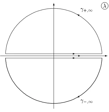
✡
Figure 1. The contoursγ±=R∪γ±∞.
Theorem 1. Let Q(x) be a potential of L which falls off fast enough for x → ±∞ and the corresponding RHP has a finite number of simple singularities at the points λ±j ∈ C±, i.e. χ±
gen(x, λ) have simple poles and zeroes at λ±j. Then
1) R±
gen(x, y, λ) is an analytic function of λfor λ∈C± having pole singularities at λ±j ∈C±;
2) R±
gen(x, y, λ) is a kernel of a bounded integral operator for Imλ6= 0;
3) Rgen(x, y, λ) is an uniformly bounded function for λ ∈ R and provides the kernel of an
unbounded integral operator; 4) R±
gen(x, y, λ) satisfy the equation:
Lgen(λ)R±gen(x, y, λ) =11δ(x−y).
Skipping the details (see [17]) we will formulate below the completeness relation for the eigenfunctions of the Lax operator Lgen. It is derived by applying the contour integration
method (see e.g. [30,1]) to the integral:
Jgen(x, y) = 1 2πi
I
γ+
dλR+gen(x, y, λ)− 1 2πi
I
γ−
dλRgen− (x, y, λ),
where the contours γ± are shown on the Fig. 1and has the form:
The explicit form of the dressing factors ugen(x, λ) makes it obvious that the kernel of the
resolvent has only simple poles atλ=λ±k. Therefore the final form of the completeness relation for the Jost solutions ofLgen takes the form [17]:
δ(x−y)
n
X
s=1
1 as
Ess
= 1 2π
Z ∞
−∞ dλ
k0 X
s=1
|χ[gens]+(x, λ)ihχˆ[gens]+(y, λ)| −
n
X
s=k0+1
|χ[gens]−(x, λ)ihχˆ[gens]−(y, λ)|
+
N
X
j=1
Res
λ=λ+j
R+(x, y) + Res
λ=λ−j
R−(x, y)
!
It is easy to check that the residues in (3.10) can be expressed by the properly normalized eigenfunctions of Lgen corresponding to the eigenvaluesλ±j [17].
Thus we conclude that the continuous spectrum ofLgen has multiplicity n and fills up the
whole real axis Rof the complexλ-plane; the discrete eigenvalues ofLgen constructed using the
dressing factors ugen(x, λ) are simple and the resolvent kernel Rgen(x, y, λ) has poles of order
one atλ=λ±k.
3.3 Resolvent and spectral decompositions for BD.I-type Lax operators
In our caseJ hasnvanishing eigenvalues which makes the problem more difficult. We can rewrite the Lax operator in the form:
i∂χ1 ∂x +~q
Tχ~
0 =λχ1,
i∂~χ0 ∂x +~q
∗χ
1+s0~qχ−1 = 0,
i∂χ−1 ∂x +~q
†s
0χ~0 =λχ−1,
where we have split the eigenfunction χ(x, λ) of L into three according to the natural block-matrix structure compatible with J: χ(x, λ) = χ1, ~χT0, χ−1T. Note that the equation for χ~0
can not be treated as eigenvalue equations; they can be formally integrated with:
~
χ0(x, λ) =χ~0,as+i Z x
dy(~q∗χ1+s0~qχ−1),
which eventually casts the Lax operator into the following integro-differential system with non-degenerate λdependence:
i∂χ1 ∂x +i~q
T(x)
Z x
dy(~q∗χ1+s0~qχ−1) (y, λ) =λχ1,
i∂χ−1 ∂x +i~q
†(x)s 0
Z x
dy(~q∗χ1+s0~qχ−1) (y, λ) =−λχ−1.
Similarly we can treat the operator which is adjoint toL whose FAS ˆχ(x, λ) are the inverse to χ(x, λ), i.e. ˆχ(x, λ) =χ−1(x, λ). Splitting each of the rows of ˆχ(x, λ) into components as follows
ˆ
χ(x, λ) = ( ˆχ1,χ~ˆ0,χˆ−1) we get:
i∂χˆ1
∂x −( ˆ~χ0, ~q ∗)
−λχˆ1 = 0,
i∂χ~ˆ0 ∂x −χˆ1~q
T −χˆ
−1~q†s0 = 0,
i∂χˆ−1
∂x −( ˆ~χ0, s0~q)−λχˆ−1 = 0.
Again the equation for ˆχ~0 can be formally integrated with:
ˆ ~
χ0(x, λ) = ˆχ~0,as+i Z x
dyχˆ1(y, λ)~qT(y) + ˆχ−1(y, λ)~q†(y)s0
.
Now we get the following integro-differential system with non-degenerate λdependence
i∂χˆ1 ∂x −i
Z x
dyχˆ1(y, λ)(~qT(y), ~q∗(x)) + ˆχ−1(y, λ)(~q†(y)s0~q∗(x))
i∂χˆ−1 ∂x −i
Z x
dyχˆ1(y, λ)(~qT(y)s0~q(x)) + ˆχ−1(y, λ)(~q†(y), ~q(x))
−λχˆ−1 = 0.
Now we are ready to generalize the standard approach to the case of BD.I-type Lax operators. The kernelR(x, y, λ) of the resolvent is given by:
R(x, y, λ) =
R+(x, y, λ) for λ∈C+,
R−(x, y, λ) for λ∈C−,
where
R±(x, y, λ) =±iχ±(x, λ)Θ±(x−y) ˆχ±(y, λ),
Θ±(z) =θ(∓z)E11−θ(±z)(11−E11).
The completeness relation for the eigenfunctions of the Lax operator L is derived by applying the contour integration method (see e.g. [30,1]) to the integral:
J′(x, y) = 1 2πi
I
γ+
dλΠ1R+(x, y, λ)−
1 2πi
I
γ−
dλΠ1R−(x, y, λ),
where the contoursγ±are shown on the Fig.1 and Π1 =E11+En+2,n+2. Using equations (3.8)
and (3.9) we are able to check that the kernel of the resolvent has poles of second order at λ=λ±k. Therefore the completeness relation takes the form:
Π1δ(x−y) =
1 2π
Z ∞
−∞ dλΠ1
n
|χ[1]+gen(x, λ)ihχˆgen[1]+(y, λ)| − |χgen[n+2]−(x, λ)ihχˆgen[n+2]−(y, λ)|o
+ 2i
N
X
j=1 (
Res
λ=λ+k
R+(x, y, λ) + Res
λ=λ−k
R−(x, y, λ) )
,
where
Res
λ=λ±k
R±(x, y, λ) =±(λ−k −λ+k)Π1
χ+,(k)(x) ˆ˙χ+,(k)(y) + ˙χ+,(k)(x) ˆχ+,(k)(y).
In other words the continuous spectrum ofLhas multiplicity 2 and fills up the whole real axisR
of the complex λ-plane; the discrete eigenvalues of L constructed using the dressing factors u(x, λ) (3.7) lead to second order poles of resolvent kernelRgen(x, y, λ) at λ=λ±k.
4
Resolvent and spectral decompositions
in the adjoint representation of
g
≃
B
rThe simplest realization of Lin the adjoint representation is to make use of the adjoint action of Q(x)−λJ ong:
Ladead ≡i
∂ead
∂x + [Q(x)−λJad, ead(x, λ)] = 0.
Note that the eigenfunctions ofLadtake values in the Lie algebrag. They are known also as the
‘squared solutions’ of L and appear in a natural way in the analysis of the transform from the potential Q(x, t) to the scattering data ofL, [1]; see also [14,17] and the numerous references therein.
the minimal sets of scattering dataTi. These ideas have been generalized also to the symmetric spaces, see [14,25,22] and the references therein.
The ‘squared solutions’ that play the role of generalized exponentials are determined by the FAS and the Cartan–Weyl basis of the corresponding algebra as follows. First we introduce:
e±α,ad(x, λ) =χ±Eαχˆ±(x, λ), e±j,ad(x, λ) =χ±Hjχˆ±(x, λ),
where χ±(x, λ) are the FAS ofL and E
α, Hj form the Cartan–Weyl basis of g. Next we note
that in the adjoint representationJad· ≡adJ· ≡[J,·] has kernel. Just like in the previous section
we have to project out that kernel, i.e. we need to introduce the projector:
πJX ≡ad−J1adJX,
for any X ∈ g. In particular, choosing g ≃so(2r+ 1) andJ as in equation (2.1) we find that the potential Qprovides a generic element of the image ofπJ, i.e.πJQ≡Q.
Next, the analysis of the Wronskian relations allows one to introduce two sets of squared solutions:
Ψ±α =πJ(χ±(x, λ)Eαχˆ±(x, λ)), Φ±α =πJ(χ±(x, λ)E−αχˆ±(x, λ)), α∈∆+1.
We remind that the set ∆1 contains all roots ofso(r+ 1) for whichα(J)6= 0.
Let us introduce the sets of ‘squared solutions’:
{Ψ}={Ψ}c∪ {Ψ}d, {Φ}={Φ}c∪ {Φ}d,
{Ψ}c≡
Ψ+α(x, λ), Ψ−−α(x, λ), i < r, λ∈R ,
{Ψ}d ≡nΨ+α;j(x), Ψ˙+α;j(x), Ψ−−α;j(x), Ψ˙−−α;j(x)oN
j=1,
{Φ}c≡Φ+−α(x, λ), Φ−α(x, λ), i < r, λ∈R ,
{Φ}d≡ n
Φ−+α;j(x), Φ˙+−α;j(x), Φ−α;j(x), Φ˙−α;j(x)oN
j=1,
where the subscripts ‘c’ and ‘d’ refer to the continuous and discrete spectrum of L.
Each of the above two sets are complete sets of functions in the space of allowed potentials. This fact can be proved by applying the contour integration method to the integral
JG(x, y) = 1 2πi
I
γ+
dλG+(x, y, λ)− 1 2πi
I
γ−
dλG−(x, y, λ),
where the Green function is defined by:
G±(x, y, λ) =G±1(x, y, λ)θ(y−x)−G±2(x, y, λ)θ(x−y), G±1(x, y, λ) = X
α∈∆+1
Ψ±±α(x, λ)⊗Φ±∓α(y, λ),
G±2(x, y, λ) = X
α∈∆0∪∆−1
Φ±±α(x, λ)⊗Ψ±∓α(y, λ) +
r
X
j=1
h±j (x, λ)⊗h±j (y, λ),
h±j (x, λ) =χ±(x, λ)Hjχˆ±(x, λ).
Skipping the details we give the result [25,27]:
δ(x−y)Π0J =
1 π
Z ∞
−∞
−2i
4.1 Expansion over the ‘squared solutions’
The completeness relation of the ‘squared solutions’ allows one to expand any function over the ‘squared solutions’
The expansions (4.2), (4.3) is another way to establish the one-to-one correspondence bet-ween Q(x) and each of the minimal sets of scattering data T1 and T2 (2.10). Likewise the expansions (4.4), (4.5) establish the one-to-one correspondence between the variation of the potentialδQ(x) and the variations of the scattering data δT1 andδT2.
The expansions (4.4), (4.5) have a special particular case when one considers the class of variations of Q(x, t) due to the evolution int. Then
δQ(x, t)≡Q(x, t+δt)−Q(x, t) = ∂Q
∂t δt+O (δt)
2.
Assuming thatδtis small and keeping only the first order terms inδtwe get the expansions for ad−J1Qt. They are obtained from (4.4), (4.5) by replacing δρ±α(λ) and δτα±(λ) by ∂tρ±α(λ) and
∂tρ±α(λ).
4.2 The generating operators
To complete the analogy between the standard Fourier transform and the expansions over the ‘squared solutions’ we need the analogs of the operator D0 =−id/dx. The operatorD0 is the
one for which eiλx is an eigenfunction: D0eiλx=λeiλx. Therefore it is natural to introduce the
generating operators Λ± through:
(Λ+−λ)Ψ+−α(x, λ) = 0, (Λ+−λ)Ψ−α(x, λ) = 0, (Λ+−λ±j)Ψ+∓α;j(x) = 0,
(Λ−−λ)Φ+α(x, λ) = 0, (Λ−−λ)Φ−−α(x, λ) = 0, (Λ+−λ±j)Φ+±α;j(x) = 0,
where the generating operators Λ± are given by:
Λ±X(x)≡ad−J1
idX dx + i
Q(x),
Z x
±∞
dy[Q(y), X(y)]
.
The rest of the squared solutions are not eigenfunctions of neither Λ+ nor Λ−:
(Λ+−λ+j ) ˙Ψ
+
−α;j(x) =Ψ+−α;j(x), (Λ+−λ−j) ˙Ψ
−
α;j(x) =Ψ−α;j(x),
(Λ−−λ+j ) ˙Φ +
ir;j(x) =Φ+α;j(x), (Λ−−λ−j) ˙Φ −
α;j(x) =Φ−α;j(x),
i.e., ˙Ψ+α;j(x) and ˙Φ+α;j(x) are adjoint eigenfunctions of Λ+ and Λ−. This means that λ±j , j =
1, . . . , N are also the discrete eigenvalues of Λ± but the corresponding eigenspaces of Λ± have
double the dimensions of the ones of L; now they are spanned by bothΨ±∓α;j(x) and ˙Ψ±∓α;j(x). Thus the sets {Ψ}and {Φ}are the complete sets of eigen- and adjoint functions of Λ+ and Λ−.
Therefore the completeness relation (4.1) can be viewed as the spectral decompositions of the recursion operators Λ±. It is also obvious that the continuous spectrum of these operators fills
up the real axis Rand has multiplicity 2n; the discrete spectrum consists of the eigenvaluesλ±
k
and each of them has multiplicity 2.
5
Resolvent and spectral decompositions
in the spinor representation of
g
≃
B
rUsing the general theory one can calculate the explicit form of the Cartan–Weyl basis in the spinor representations. In Appendices Band Cbelow we give the results for r = 2 and r = 3. Therefore in the spinor representation the Lax operators take the form:
Lspψsp=i
∂ψsp
where Qsp(x, t) and Jsp are 2r×2r matrices of the form: It is well known [5] that the spinor representations of so(2r+ 1) are realized by symplectic (resp. orthogonal) matrices if r(r + 1)/2 is odd (resp. even). Thus in what follows we will view the spinor representations ofso(2r+ 1) as typical representations of sp(2r) (resp. so(2r))
algebra. Combined with the corresponding value of Jsp (B.1) one can conclude that that the
Lax operator Lspfor odd values ofr(r+ 1)/2 can be related to the C.III-type symmetric spaces.
The potentialQsp(x) however is not a generic one; it may be obtained from the generic potential
as a special reduction, which picks up so(2r+ 1) as the subalgebra of sp(2r). Below we will construct an automorphism whose kernel will pick up so(2r+ 1) as a subalgebra of sp(2r).
Similarly the Lax operator Lsp above for even values of r(r + 1)/2 can be related to the
so(2r) algebra. The element Jsp (B.1) is characteristic for the D.III-type symmetric spaces.
The potential Qsp(x) may be obtained from the generic potential as a special reduction, which
picks up so(2r+ 1) as the subalgebra ofso(2r).
The spectral problem (5.1) is technically more simple to treat. It has the form of block-matrix AKNS which means that the corresponding Jost solutions and FAS are determined as follows:
ψ(x, λ) ≃
5.1 The Gauss factors in the spinor representation
The spectral theory of the Lax operators related to the symmetric spaces of C.III and D.III types were developed in [20, 28]. What is different here is the special choice of the rank and the additional reduction πBr which picks up the spinor representation of so(2r+ 1). In our
considerations below we will assume that this reduction is applied. So though all our 2r×2r
matrices are split into blocks of dimension 2r−1×2r−1, the corresponding group (resp. algebraic)
elements belong to the (spinor representation of) group SO(2r+ 1) (resp. algebraso(2r+ 1)). Thus we define the FAS ofLsp by:
sp(λ) are block-diagonal and equal:
D+sp(λ) =
All factorsS±sp,T±spand D±
sp take values in the spinor representation of the groupSO(2r+ 1)
and are determined by the minimal sets of scattering data (2.15). Besides, since
Tsp(λ) =T−sp(λ)Dsp+(λ) ˆS
Strictly speaking it isX±
sp(x, λ) that allow analytic extension forλ∈C±. They have also another
nice property, namely their asymptotic behavior for λ→ ±∞ is given by:
lim
Equations (5.8) combined with (5.7) are known as a Riemann–Hilbert problem (RHP) with ca-nonical normalization [13]. It has unique regular solution; the matrix-valued solutionsX0+,sp(x, λ) and X0−,sp(x, λ) of (5.8), (5.7) is called regular if detX0±,sp(x, λ) does not vanish for anyλ∈C±.
Equations (5.9), (5.10) can be viewed as a set of singular integral equations which are equivalent to the RHP. For the MNLS these were first derived in [40].
Finally, the potentialQ(x, t) can be recovered from the solutionsXsp±(x, λ) of RHP (5.8) with a canonical normalisation (5.7). Skipping the details, we provide here only the final result:
Qsp(x, t) = lim
λ→∞λ(J −X ±
sp(x, λ)JXˆsp±(x, λ)]) = [J, X1(x)],
where X1(x) = lim
λ→∞(Xsp(x, λ)−11).
5.2 Def inition and properties of R±sp(x, y, λ)
The resolvent Rsp(λ) ofLsp is again expressed through the FAS in the form:
Rsp(λ)f(x) = Z ∞
−∞
Rsp(x, y, λ)f(y),
where Rsp(x, y, λ) are given by:
Rsp(x, y, λ) =
R+sp(x, y, λ) for λ∈C+, R−
sp(x, y, λ) for λ∈C−,
and
R±sp(x, y, λ) =±iχ±sp(x, λ)Θ±(x−y) ˆχ±sp(y, λ), Θ±(z) =
θ(∓z)11 0 0 −θ(±z)11
.
5.3 The dressing factors in the spinor representation
The asymptotics of the dressing factor forx→ ±∞ are:
u±= exp (lnc1(λ)Jsp),
where
u+=
√
c1112r 0
0 1/√c1112r−1
, u− =
1/√c1112r−1 0
0 √c1112r−1
.
Thus the asymptotics of the projectors P and ¯P in the spinor representation are projectors of rank 2r−1. Since the dynamics of the MNLS does not change the rank of the projectors we
conclude that the dressing factor in the spinor representation must be of the form:
u(x, λ) = exp
1
2lnc1(λ)(P1−P¯1)
=pc1(λ)P1(x, t) +
1
p
c1(λ)
¯ P1(x, t)
dressing factors of such form with non-rational dependence on λ were considered for the first time in by Ivanov [35] for the MNLS related to symplectic algebras. Here we see that such construction can be used also for the orthogonal algebras.
However when it comes to analyze the relations between the ‘naked’ and the dressed scattering matrices and their Gauss factors we get integer powers of c1(λ). Indeed, for the simplest case
when the dressing procedure is applied just once we have:
and as a consequence
a+sp(λ) = 1 c+1(λ)a
+
0,sp(λ), a−sp(λ) =c+1(λ)a−0,sp(λ),
ρ+sp(λ) = 1 c+1(λ)ρ
+
0,sp(λ), ρ−sp(λ) =c+1(λ)ρ−0,sp(λ),
τsp+(λ) = 1 c+1(λ)τ
+
0,sp(λ), τsp−(λ) =c+1(λ)τ0−,sp(λ).
5.4 The spectral decompositions of Lsp
Again apply the contour integration method to the kernel R±
sp and derive the following
com-pleteness relation:
δ(x−y)112r = 1
2π
Z ∞
−∞
dλ|φ+(x, λ)iaˆ+(λ)hψ+(y, λ)| − |φ−(x, λ)iaˆ−(λ)hψ−(y, λ)|
+
N
X
j=1
Res
λ=λ+j
R+(x, y) + Res
λ=λ−j
R−(x, y) !
. (5.11)
The residues in (5.11) can be expressed by the properly normalized eigenfunctions ofLsp
corre-sponding to the eigenvalues λ±j .
Thus we conclude that the continuous spectrum of Lsp fills up R and has multiplicity 2r.
The discrete eigenvalues λ±k are simple poles of the resolvent.
6
Dressing factors and higher representations of
g
Here we will briefly outline how, starting from equation (2.13) one can construct the dressing factors in any irreducible representation of the Lie algebra g. We will illustrate this on one of the simple nontrivial examples of u(x, λ) with rank-1 projectors P(x) and ¯P(x). Our intention is to outline the explicit λ-dependence of u(x, λ) in any IRREP. To this end it will be most convenient to use the first line of equation (3.1):
u(x, λ) = exp lnc1(λ)(P1−P¯1). (6.1)
Note that P(x)−P¯(x)∈g and therefore the right hand side of (6.1) will be an a Lie group ele-ment. In what follows we will assume that rankP(x) = rank ¯P(x) = 1 and will derive explicitly theλ-dependence of the right hand side of equation (6.1) in any irreducible representation of g. In fact it will be enough to analyze theλ-dependence of the asymptotic ofu(x, λ) forx→ ±∞.
lim
x→∞(P(x)−
¯
P(x)) =He1.
In order to be more specific we will do our considerations for the case when f ≃ so(7). This algebra is of rank 3. We also choose the representation with highest weight
ω= 3ω3 =
3
2(e1+e2+e3).
The structure of the weight system Γ(ω) is described in Table1.
It is natural to expect that u(x, λ) will have the same type of λ-dependence [15] as its asymptotic for x → ±∞. Therefore we will evaluate the right hand side of equation (6.1) for x→ ∞. Doing this we well use the known formula
He1 = X
γ∈Γ(3ω3)
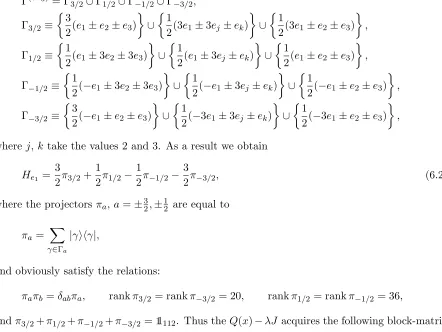
Table 1. The structure of the weight system Γ(3ω1)
for the algebraso(7) with dimension 112. We list here the number of weights of different lengthsℓ(γ) and their multiplicityµ(γ) and length. The indices i, j,kare different and take values 1, 2 and 3.
Therefore we have to arrange the weights in Γ(3ω3) according to their scalar products with e 1,
Inserting equation (6.2) into equation (6.1) we get:
lim
x→∞u
(3ω3)(x, λ) = (c(λ))3/2π
3/2+ (c(λ))1/2π1/2+ (c(λ))−1/2π−1/2+ (c(λ))−3/2π−3/2,
and as a result for the λ-dependence of u(3ω3)(x, λ) and its inverse we get:
u(3ω3)(x, λ) = (c(λ))3/2π
3/2(x) + (c(λ))1/2π1/2(x)
+ (c(λ))−1/2π−1/2(x) + (c(λ))−3/2π−3/2(x),
(u(3ω3))−1(x, λ) = (c(λ))−3/2π
3/2(x) + (c(λ))−1/2π1/2(x)
+ (c(λ))1/2π−1/2(x) + (c(λ))3/2π−3/2(x).
The four projectors πa(x) have the same properties as their asymptotic values:
πa(x)πb(x) =δabπa(x),
rankπ3/2(x) = rankπ−3/2(x) = 20, rankπ1/2(x) = rankπ−1/2(x) = 36.
Their explicit x dependence as well as the interrelation between the potentials Q(0)(x) and Q(1)(x) follow from the equation for u(x, λ) (2.12) considered in the representationV(3ω3). In
particular we get:
Q(1)(x)−Q(0)(x) = lim
λ→∞λ
J−u(3ω3)J(u(3ω3))−1(x, λ)
= (λ+−λ−)
J,3
2(π3/2(x)−π−3/2(x)) + 1
2(π1/2(x)−π−1/2(x))
.
Though the expressions for the dressing factor in this representation seem to be rather complex, nevertheless they are determined uniquely by the projector P1(x), or equivalently, through the
polarization vector|n1(x)i. The corresponding expressions can be using the fact thatV(3ω3)can
be extracted as the invariant subspace of the tensor productV(ω3)⊗V(ω3)⊗V(ω3)corresponding
to the highest weight vector 3ω3. Therefore one can conclude that the matrix elements of the
projectorsπa,a=±3/2,±1/2 will be polynomials of sixth order of the components of |n1(x)i.
Our final remark concerns the analyticity properties of the FAS dressed by u(3ω3)(x, λ).
The factor itself contains powers of root square of c(λ) which in general may lead to essential singularities at λ=λ+ and λ=λ−. Note however that the dressed FAS in this representation
are obtained from the regular solutions via the analog of equation (2.11):
χ±,3ω3
1 (x, t, λ) =u(3ω3)(x, λ)χ ±,3ω3
0 (x, t, λ)(u3−ω3)−1(λ), u3ω3
− (λ) = limx→−∞u3ω3(x, λ) = exp (−lnc1(λ)He1)
= (c(λ))3/2π=3/2+ (c(λ))1/2π−1/2+ (c(λ))−1/2π1/2+ (c(λ))−3/2π3/2. (6.3)
It is not difficult to check that the right hand side of first line in equation (6.3) does not contain square root terms of c(λ); all half-integer powers of c(λ) get multiplied by other half-integer powers and the result is thatχ±,3ω3
1 (x, t, λ) acquires additional pole singularities atλ=λ+ and
λ=λ−.
7
Conclusions
We have analyzed the spectral properties of the Lax operators related to three different repre-sentations of g ≃Br: the typical, the adjoint and the spinor representation. In all these cases
eigenvalues; ii) the explicit form of the dressing factors; iii) the completeness relations of the eigenfunctions are substantially different. However the minimal sets of scattering data Ti are
provided by the same sets of functions, i.e. the sets Ti are invariant with respect to the choice
of the representation of g.
Our considerations were performed for the class of smooth potentials Q(x) vanishing fast enough for x → ±∞. Similar results can be derived also for the class of potentials tending to constants Q± forx→ ±∞.
A
The adjoint representations of
so
(5) and
so
(7)
The adjoint representations of all orthogonal algebras so(2r+ 1) and so(2r) are characterized by the fundamental weight ω2=e1+e2. By definition the corresponding weight system is
Γω2 ≡∆∪ {0}r,
where ∆ is the root system of the algebra and{0}is a vanishing weight with multiplicityr. We will order the weights in Γω2 according to their scalar products with e1.
Let us consider in more detail the two special cases ofso(2r+ 1) with r = 2 andr = 3. For r = 2 the adjoint representation is 10-dimensional. Ordering the roots as mentioned above we get:
∆+1 ≃ {e1+e2, e1, e1−e2}, ∆0 ≃ {e2,−e2}, ∆−1 ≃ {−e1+e2, e1,−e1−e2},
As a result the elementJ in the adjoint representation takes the form:
Jad =
112 0 0
0 06 0
0 0 −112
, Qad =
0 Qad;12 0
Qad;21 06 Qad;23
0 Qad;32 0 .
Analogously for r = 3 the adjoint representation is 21-dimensional. Ordering the roots as mentioned above we get:
∆+1 ≃ {e1+e2, e1+e3, e1, e1−e3, e1−e2}, ∆0≃ {e2±e3,−(e2±e3)},
∆−1 ≃ {−e1+e2,−e1+e3, e1,−e1−e3,−e1−e2}.
As a result the elementJ in the adjoint representation takes the form:
Jad =
115 0 0
0 011 0
0 0 −115
, Qad =
0 Qad;12 0
Qad;21 011 Qad;23
0 Qad;32 0 .
It is not difficult to write down the explicit form ofQad but it will not be necessary. We have
used above a more compact realization of Qad as adQ.
B
The spinor representation of
so
(5)
The highest weight and the weight system of so(5) are given by [5, 33]. It is well known that so(5)≃sp(4) so the spinor representation of so(5) is realized through symplecticsp(4) matrices
ω2 ≡γ1= 1
2(e1+e2), γ2 = 1
The Cartan–Weyl basis ofso(5) is given by
Ee1−e2 = Γ2,¯2 =E2ǫ2, Ee1+e2 = Γ1,¯1=E2ǫ1, Ee1 = Γ1,¯2−Γ2,¯1 =Eǫ1+ǫ2, Ee2 = Γ1,2−Γ2,¯1=Eǫ1−ǫ2,
He1 =
1
2(Γ1,1+ Γ2,2), He2 =
1
2(Γ1,1−Γ2,2), where ¯k= 5−kand
Γk,p =|γkihγp|, 1≤k≤p≤4.
ByEǫi±ǫj above we have denoted the Weyl generators ofsp(4). The Lax operatorLin the spinor representation of so(5) takes the form:
Lspψsp=i
∂ψsp
∂x + (Qsp−λJsp)ψsp(x, λ) = 0,
where Qsp(x, t) and Jsp are 4×4 symplectic matrices of the form:
Qsp=
0 q q† 0
, Jsp=
1 2
112 0
0 −112
, q(x, t) =
q0 q¯1
q1 −q0
. (B.1)
C
The spinor representation of
so
(7)
The highest weight and the weight system of so(7) are given by [5,33]
ω3 ≡γ1= 1
2(e1+e2+e3), γ2 = 1
2(e1+e2−e3), γ3=
1
2(e1−e2+e3), γ4 = 1
2(e1−e2−e3), γ5=−γ4, γ6 =−γ3, γ7 =−γ2, γ8=−γ1.
The Cartan–Weyl basis ofso(7) is given by
Ee1−e2 = Γ3,¯4 =Eǫ3+ǫ4, Ee2−e3 = Γ2,3 =Eǫ2−ǫ3, Ee1−e3 = Γ2,4¯ =Eǫ2+ǫ4, Ee1+e2 = Γ1,2¯ =Eǫ2+ǫ4, Ee1+e3 = Γ1,¯3 =Eǫ1+ǫ3, Ee2+e3 = Γ1,4 =Eǫ1−ǫ4,
Ee1 = Γ1,¯4+ Γ2,¯3 =Eǫ1+ǫ4 +Eǫ2+ǫ3, Ee2 = Γ1,3+ Γ2,4 =Eǫ1−ǫ4 +Eǫ2−ǫ4,
Ee3 = Γ1,2−Γ3,4 =Eǫ1−ǫ2 −Eǫ3−ǫ4, He1 =
1
2(Γ1,1+ Γ2,2+ Γ3,3+ Γ4,4), He1 =
1
2(Γ1,1+ Γ2,2−Γ3,3−Γ4,4), He1 =
1
2(Γ1,1−Γ2,2+ Γ3,3−Γ4,4), where ¯k= 9−kand
Γk,p =|γkihγp| −(−1)k+p|γp¯ihγk¯|, 1≤k≤p≤4,
Γk,p¯=|γkihγp|+ (−1)k+p|γp¯ihγk¯|, 1≤k≤p≤4.
Note that the typical representation of so(8) is also 8-dimensional. So by Eǫi±ǫj above we have
reflection) which changesǫ4 ↔ −ǫ4. In short the Lax operatorLin the spinor representation of
so(7) take the form:
Lspψsp=i
∂ψsp
∂x + (Qsp−λJsp)ψsp(x, λ) = 0, where Qsp(x, t) and Jsp are 8×8 matrices of the form:
Qsp=
0 q q† 0
, Jsp=
1 2
114 0
0 −114
, q(x, t) =
q0 q¯2 q¯1 0
q2 q0 0 −q¯1
q1 0 −q0 q¯2
0 −q1 q2 −q0
. (C.1)
Our final remark here concerns the spinor representation with highest weight ω= 3ω3. Then
Γ≃
3
2(±e1±e2±e3), 1
2(±e1±e2±e3)
.
The dimension of this representation is 8. The explicit form of the elementJ in this representa-tion isJ = diag (3211,1211,−3211,−1211), i.e. all eigenvalues ofJ are non-vanishing. The potentialQ will have block-matrix structure compatible with the one ofJ.
Acknowledgements
The authors have the pleasure to thank Prof. Adrian Constantin, Prof. Nikolay Kostov, Prof. Alexander Mikhailov and Dr. Rossen Ivanov for numerous useful discussions. Part of the work was done during authors visit at the Erwin Schr¨odinger International Institute for Mathematical Physics in the framework of the research programme “Recent Advances in Integrable Systems of Hydrodynamic Type” (October 2009). One of us (GGG) is grateful to the organizers of the Kyiv conference for their hospitality. This material is based upon works supported by the Science Foundation of Ireland (SFI), under Grant No. 09/RFP/MTH2144. We thank three anonymous referees for numerous useful suggestions.
References
[1] Ablowitz M.J., Kaup D.J., Newell A.C., Segur H., The inverse scattering transform – Fourier analysis for nonlinear problems,Studies in Appl. Math.53(1974), 249–315.
[2] Ablowitz M.J., Prinari B., Trubatch A.D. Discrete and continuous nonlinear Schr¨odinger systems,London Mathematical Society Lecture Note Series, Vol. 302, Cambridge University Press, Cambridge, 2004.
[3] Athorne C., Fordy A., Generalised KdV and MKDV equations associated with symmetric spaces,J. Phys. A: Math. Gen.20(1987), 1377–1386.
[4] Beals R., Sattinger D.H., On the complete integrability of completely integrable systems, Comm. Math. Phys.138(1991), 409–436.
[5] Bourbaki N., ´El´ements de math´ematique,Actualit´es Scientifiques et Industrielles, no. 1364, Hermann, Paris, 1975 (in French).
[6] Calogero F., Degasperis A., Spectral transform and solitons, Vol. I, North-Holland Publishing Co., Amster-dam – New York, 1982.
[7] Calogero F., Degasperis A., Nonlinear evolution equations solvable by the inverse spectral transform. I,
Nuovo Cimento B32(1976), 201–242.
Calogero F., Degasperis A., Nonlinear evolution equations solvable by the inverse spectral transform. II,
Nuovo Cimento B39(1976), 1–54.