6.1 6.2 6.3 6.4 6.5 6.6 6.7
6.1
6.2
INTRODUCTION
RANDOM VARIABLES
INTRODUCTIONRANDOM VARIABLES
DISCRETE PROBABILITY DISTRIBUTIONS MEAN AND VARIANCE
THE BINOMIAL PROBABILITY DISTRIBUTION USING MINITAB (OPTIONAL)
SUMMARY
REVIEW EXERCISES
random variables,
probability distributions,
6
CHAPTER
PROBABILITY DISTRIBUTIONS FOR
DISCRETE RANDOM VARIABLES
In Chapters 2 and 3, we were concerned with the analysis of numerical data. In Chapter 5, we studied the concepts of experiment, outcome, sample space, and probability. In this chapter, we bring these ideas together by introducing
which describe numerical properties of the elements of a sample space. In this text, we will ultimately be interested in the study of populations. We will
see that which are studied in this chapter and Chapter 7,
can be used to summarize the essential features of a population of data values.
Outcome
Number of Yes Responses 4
random variable
occurred
YN.
S YN, NY, YY, NN
random variable.
Definition
EXAMPLE 6.1
EXAMPLE 6.2
In any scientific inquiry, it is helpful to translate that which is being studied into numbers. For instance, if we are interested in the fuel efficiency of various kinds of automobiles, we would look at the mileage rating (number of miles per gallon of fuel) for each kind of car. The process of assigning numbers to the objects being studied seems to be a natural one.
Given a sample space, we often study some numerical property of the various outcomes in the sample space. For example, consider the collection of adult Ameri-cans. (This is the sample space associated with the experiment of selecting an adult American at random.) One possible numerical property of interest might be the age of each person. Once we have specified the numerical property of interest, we have in essence given a rule for assigning a certain number to each element of the sample space. (Next to the name of each adult American, we assign the number that represents that person’s age.) A rule for assigning such numbers is called a
A rule that enables us to assign a number to each outcome of a sample space is called a on the sample space. The actual number associated with a particular outcome is called the value (or data value) of the random variable associated with this outcome. When the experiment is performed, the value associated with the outcome is said to have or been observed.
In the 1992 presidential election, a pollster was assigned to interview the oldest male and female in various households. Each was asked whether he or she voted for George Bush. If the male said “Yes” and the female said “No,” the pollster recorded The interview of one household can be viewed as an experiment with sample space
Consider the random variable “number of yes responses” from the two voters. The possible values are 0, 1, and 2, as shown in the following table:
Consider the collection (sample space) of all working people in the United States. We could consider a number of random variables, such as weight, height, age, salary, and so on.
h j
YN NY YY NN
4 4
x y z
x
x x
x
x
x
x
y y
y
continuous
discrete
interval line
segment. continuous
discrete
Definitions
probability distribution
We often use a symbol such as , , or to represent an arbitrary or unspecified value of a random variable. Thus in Example 6.1, we could have used to represent any one of the values 0, 1, or 2. We could also use the symbol more abstractly to represent the random variable itself. Thus we could say: Consider the random variable , where the number of yes responses.
Suppose we let the water temperature at some randomly selected point in Lake Erie next September 1. Then could potentially be any value between freezing (32 F) and boiling (212 F). (A spot containing industrial waste might account for the possibility of extremely high temperatures.)
32 F 212 F
This inequality says that must be greater than 32 F and less than 212 F. The numbers that satisfy this inequality constitute what is called an or
The random variable “Water temperature” is a random
variable; it can potentially assume any value on an interval [Figure 6.1(a)].
On the other hand, suppose that we select three light bulbs from a production line. Let be the random variable that counts the number of defectives. So can potentially assume any one of the values 0, 1, 2, or 3. We call a random variable; the values it can potentially assume constitute separated or isolated points on the real number axis. For example, we could get 1 or 2 defectives but not 1.5 defectives. See Figure 6.1(b).
A random variable is if it potentially can take on any value on some line segment or interval (that is, there are no “breaks” between possible values). A random variable is if the values it can potentially assume constitute a sequence of isolated or separated points on the real number axis.
Continuous random variables usually measure the amount of something, whereas discrete random variables usually count something.
Here are some additional examples of continuous random variables: a person’s height, the length of time to run a marathon, the mass in kilograms of a celestial object (planet, star, meteor, piece of space dust, etc.). In this last example, we would consider the mass to be theoretically any value greater than 0, showing that sometimes the interval of possible values of a random variable is considered to be infinite in length.
Additional examples of discrete random variables are the number of children in a family, the number of times a person catches a cold in a given year, and the number of tosses of a coin before a tail appears. This last example shows that sometimes the sequence of potential values of a discrete random variable can be infinite because the sequence in this example would be 1, 2, 3, . . . .
We will ultimately be interested in probabilities associated with various values of a random variable. A formula or table that enables us to find such probabilities is called a for the random variable. We investigate probability distributions for discrete random variables in this chapter. In Chapter 7, we will study probability distributions for continuous random variables.
8
8
8
8
8
8
6.1 (a) (b) (c) (d) (e) (f) 6.2
(a) (b) 6.3
(a) (b) (c) 6.4
(a) (b) 6.5
(a) (b) 6.6
(a) (b) 6.7
(a) (b) 6.8
(a) (b)
4 4 4
4
4
4
4 4
EXERCISES
x
x x
x
x x x
x
x x
x x x
x
x x
x x
Classify the following random variables as discrete or continuous: The number of automobile fatalities over a 72-hour period The length of time to run a 100-yard dash
The diameter of pebbles from a stream
The number of incoming phone calls to a switchboard at a city hospital The barometric pressure at noon at a specific location
The number of bills paid on time per month to a plumber
One word is randomly selected from the following sentence: The grass needs cutting and should be cut by tomorrow afternoon. Let be the number of letters in the selected word.
What values can assume?
Is a discrete or continuous random variable?
A green, a red, and a blue die are tossed. In each of the following, find the values that can assume:
Let the sum of the three dice.
Let the minimum number of dots showing on any die. Let two times the number of dots on the green die.
One hundred voters in a suburban town are to be selected and asked whether they approve of a civic arena being built. Let the number of voters in the sample who approve.
What values can assume?
Is a discrete or continuous random variable?
A manufacturer of light bulbs is interested in various properties about the length of life of his product. Let length of life of a light bulb (measured in hours).
What values can assume?
Is a discrete or continuous random variable?
An engineer is testing samples of steel cables to be used in the construction of a suspension bridge.
Describe one random variable of possible interest. Is the random variable discrete or continuous?
A health official wanted to investigate the relationship between females with no children and the incidence of breast cancer. Five hundred women, 40–45 years of age, with no children and no prior breast cancer, are selected. Let the number of women who develop breast cancer during the following 5 years.
What values can assume?
Is a discrete or continuous random variable?
A known health effect associated with exposure to elevated levels of radon is an increased risk of developing lung cancer. The alpha track detector is a device for measuring the amount of radon in the air. The amount is measured in picocuries of radon per liter of air (pCi/l). The Environmental Protection Agency (EPA) action level for radon in air is 4.0 pCi/l. An alpha track detector is placed in the cellars of 50 randomly selected homes. Classify the random variable in parts (a) and (b) as continuous or discrete, and state the values it can assume.
Let the mean pCi/l level of the 50 measurements.
6.3
DISCRETE PROBABILITY DISTRIBUTIONS
4
4
4 4
4 4
4 ,
x ,
B G
S B, G
x x
x x
P P
discrete probability
distribution. x
P x
x
x x
x x
CW probability distribution.
Definition
EXAMPLE 6.3
Solution
In a study of families with one child, a researcher coded families as follows: 0 if child is a boy
1 if child is a girl
Imagine the experiment of randomly selecting a family with one child and recording whether the child is a boy ( ) or a girl ( ). The sample space is
and is a random variable on this sample space. We can view as the number of girls in a randomly selected family with one child (0 or 1). We assume that a boy and a girl are equally likely. Hence, the probability that 0 (a boy) is and the probability that 1 (a girl) is . We sometimes write
(0) (1)
The specification of the probabilities associated with the distinct values of this
random variable is called its We generalize this idea with
the following definition.
The specification of the probabilities associated with the various distinct values of a discrete random variable is called a
The probability associated with the value is denoted by the symbol ( ).
If many one-child families were selected, and the number of girls (0 or 1) were recorded for each family, a population of data values would be generated. The probability distribution for (the number of girls) provides a theoretical description of what this population should look like: Since the probability of observing a 0 is and the probability of observing a 1 is , the 0’s and 1’s should occur in equal proportions (in the long run).
It is often convenient to think of a conceptual population of data values associated with a random variable . This is the collection of values that would result if the experiment were performed many times. Sometimes we imagine the experiment as being performed repeatedly for an unlimited number of times. In this case, the population is viewed as infinite, because there is no reason to impose a specific limit on the number of times the experiment is performed.
In Chapter 5, we discussed the experiment where a student randomly guesses at the two questions on a true–false quiz. Let the number of correct guesses. Find the probability distribution for .
Recall that correct on the first question and wrong on the second is . The sample space associated with the experiment of taking the quiz by guessing is
1 2 1
2
1 1
2 2
1 1
2 2
h j
Outcome
( )
1 4 1 2 1 4
4
4 4
4 4 ` 4
4 4
4
4
S CW, WC, WW, CC
S
x
WW
P P WW
CW WC CW, WC
P P CW, WC
CC
P P CC
x
x x
P EXAMPLE 6.4
Solution
x
x P x
Each outcome in is equally likely. Therefore, each has the probability . The values of the random variable are given by the following table:
The value 0 will occur if occurs. Thus
(0) ( )
The value 1 will occur if either or occurs—that is, if the event occurs:
(1) ( )
The value 2 will occur if occurs. Therefore
(2) ( )
The probability distribution is summarized in the following table:
where is the number of correct guesses.
A college statistics class has 20 students. The ages of these students are as follows: One student is 16 years old, four are 18, nine are 19, three are 20, two are 21, and one is 30. Let the age of any student (randomly selected). Find the probability distribution for .
Since each student has an equal likelihood of being selected, the probability of selecting a particular student is . The probability of selecting a student that is 19 years old is (19) , since there are nine students of that age. The probability distribution is summarized in the following table:
1 4
1 4
1 1 1 4 4 2
1 4
1 20 9
20
h j
h j
h j
CW WC WW CC
1 1 0 2
1 20
4 20
9 20
3 20
2 20
1 20
4
4 4
4 4
4 4 4 4 4 `
4 `
4 4 4 `
4 4
P x
P x
P x x
P x
P x or x x
WW x CW WC x
x WW, CW, WC
P x or x P WW, CW, WC
P P
P x a or x b P a P b
x P x
x
P x
x
P x x , ,
EXAMPLE 6.5
x P(x)
In reading the preceding examples, you may have noted the following proper-ties, which generalize to all discrete probability distributions.
1. Since ( ) is a probability, it will always be a number between 0 and 1 inclusive:
0 ( ) 1
2. The sum of the values of ( ) for each distinct value of is 1: ( ) 1
Another point worth noting is this: Suppose in Example 6.3 that we were interested in the probability that the number of correct guesses on the two-question quiz is either 0 or 1. We write this probability as ( 0 1). Now will be 0 for two wrong guesses, , and will be 1 with the guesses or . So 0
or 1 corresponds to the event . Notice that
( 0 1) ( )
(0) (1) This result generalizes to any discrete distribution:
( ) ( ) ( )
Every discrete probability distribution must satisfy properties 1 and 2 in the preceding box. Conversely, if we are given values for and ( ) such that properties 1 and 2 are satisfied, then these values define a discrete probability distribution for some random variable . The following example illustrates this point.
Consider the expression ( ) defined by the equation
( ) for 1 2 3
6
3 1 1 4 4 2
h j
h j
^
16 18 19 20 21 30
( )
1 4 1 2 1 4
4
4 ` `
4 ` ` 4
4 P x
P x
P x
x , ,
P x P P P
P x
x P x x
x
x
P x x
x (a)
(b)
Solution (a)
(1) (2)
(b)
probability histogram.
EXAMPLE 6.6
Solution
Remark
Graphic Representations
x P x
Show that ( ) defines a probability distribution:
Give an example of an experiment, a sample space, and a random variable on the sample space for which ( ) is the probability distribution.
To show that ( ) is a probability distribution, we need only show that the two basic properties of a distribution are satisfied.
Clearly, 0 1 for 1 2 3.
( ) (1) (2) (3)
1
Therefore, ( ) is a probability distribution.
Construct an experiment and sample space as follows: Place six balls in a box. Label one ball with the number 1, label two balls with the number 2, and three balls with the number 3. Let the experiment be to select a ball at random. The sample space consists of the six balls. For the random variable, we would let be the number on the ball selected. It should be clear that ( ) /6 gives the probability associated with each value of .
We can represent a probability distribution graphically by constructing a type of
bar graph called a This is constructed by displaying the
possible distinct values of the random variable along a horizontal axis. Above each value of the random variable, we draw a vertical bar having height equal to the probability ( ). We will restrict our attention to those cases where the possible values of are whole numbers. In such cases, we make the width of each bar 1.
Construct a probability histogram for the distribution of Example 6.3.
The probability distribution is given by
The probability histogram is shown in Figure 6.2.
In Example 6.6, notice that the probability associated with a value is not 6
1 2 3 6 6 6
^
0 1 2 x
6.9
6.10
6.11
Number of Libraries Range of Holdings
6.12
6.13
Number Did Not
Number Voted Vote
Males
Females
4 x x
P x x
4
4 4
EXERCISES
x
only the height of the bar above , but it is also equal to the area of the bar above , since the width of each bar is 1. That is,
( ) area of the bar above
This will be the case for all discrete distributions we consider. This seemingly insignificant observation will be of great importance in future applications.
x x
x x
Source: The 1994 Information Please Almanac, x
x
Note:
x
x x
x
An electronics firm employs 15 people whose yearly salaries (in thousands of dollars) are
25.0 25.7 25.7 26.6 27.2 27.3 27.3 27.3 27.3 27.8 27.8 28.4 28.4 29.0 29.0
Let be the yearly salary for any employee. Find the probability distribution for . Ten thousand Instant Money lottery tickets were sold. One ticket has a face value of $1000, five tickets have face values of $500 each, 20 tickets are worth $100 each, 500 are worth $1 each, and the rest are losers. Let the value of a ticket that you buy. Find the probability distribution for .
The following table gives information on the range of holdings for 50 major U.S. college and university libraries in 1991–1992 (
1994, p. 864). The value of gives a code for each range, with 1 representing the lowest range, and 9 representing the highest range. Find the probability distribution of .
20 2–3 million 1
12 3–4 million 2
4 4–5 million 3
5 5–6 million 4
5 6–7 million 5
1 7–8 million 6
1 8–9 million 7
1 9–10 million 8
1 10 million or more 9
2–3 million means at least 2 million and less than 3 million.
A box has five tickets numbered 1, 2, 3, 4, and 5. Two are to be randomly selected without replacement. Let be the number of occurrences of either 4 or 5. For example, if 2 and 5 are selected, then 1. If both 4 and 5 are selected, then 2. Find the probability distribution for .
The following data are characteristics of the voting-age population regarding the 1992 presidential election in the United States. Number of persons is measured in thousands.
53,312 35,245
(a)
(b)
6.14
Category Frequency
6.15
In Exercises 6.16–6.19, determine whether each is a probability distribution. Give reasons for your answer.
6.16 6.17 6.18 6.19
( ) ( ) ( ) ( )
6.20
( )
1 2 1 2
2 5 3 3
1 2 1 1
4 5 3 6
1 2 1 1
2 5 3 6
1 5
1 36
3 36
5 36
7 36
9 36 11 36
4 4
4 4
4
x P x x P x x P x x P x
x P x
2
2
2
x
x x
x x
x
x
x
x
Find the probability distribution of in parts (a) and (b):
A name is to be randomly selected from those who voted. Let 0 if a male is selected. Otherwise, let 1.
A name is to be randomly selected from the female voting-age population. Let 0 if the selected female voted. Otherwise, let 1.
For adults without known heart disease, a desirable total cholesterol level is less than 200. Between 200 and 239 is categorized as borderline, and above 239 is too high. The following data are from a sample of 825 participants in the Framingham Heart Study with no prior heart disease:
Desirable 234 Borderline 297 Too high 294
Let equal 1, 2, or 3 for desirable, borderline, or too high, respectively. Find the probability distribution for .
In a population of 3000 people, 1470 were classified as blood type O, 1140 as type A, 300 as type B, and the remaining as type AB. Let 0, 1, 2, or 3 if a person’s blood type is O, A, B, or AB, respectively. Find the probability distribution for .
2 3 3 0
4 9 1 1
6 11 5 2
13
The probability distribution for the number of electronic instruments produced per hour by an assembly line is as follows:
6.4
MEAN AND VARIANCE
6.21( )
Number
Correct Frequency
1 4 1 2 1 4
4
4 x
x
N , x
P x
4
4
x P x
x
In Example 6.3, we discussed an experiment that consisted of a student randomly guessing at the answers to a two-question true–false quiz. The random variable was number of correct guesses (0, 1, or 2). The probability distribution was given by
The population for this random variable would be the string of values of that would occur if this experiment were performed over and over by many students. The probability distribution provides a theoretical description of this population, and we ought to be able to use it to predict the mean and variance of all these values.
We will try to simulate this population by considering what the data values should theoretically look like if the experiment is performed by a large number of students, say 40 000 students, and the number of correct guesses is recorded for each student. Examining the probability distribution ( ), we see that in an ideal situation we should expect 0 to occur about of the time. Thus we expect about 10,000 zeros. Similarly, we expect about 20,000 ones and 10,000 twos.
Therefore, we expect the mean of all these values to be 1
4
x
Construct a probability histogram.
A business executive was sensitive to the possibility of being accused of religious discrimination in his hiring practices. He found that of 600 employees, 204 were Catholic, 228 were Protestant, 72 were Jewish, with the rest classified as Other. Let 0, 1, 2, or 3 if a person’s religion is Catholic, Protestant, Jewish, or Other, respectively. Find the probability distribution and construct the probability histogram.
0 1 2
0 10,000
1 20,000
4
` `
4
4 ` `
4 ` ` 4
4 4 4
4 ` ` 4
4
4
4 x N
, , ,
,
, , ,
, , ,
P P P
P P P
x P x x
x P x
N N
x
P x mean x
x P x
Note: P x
P x
x x
x P x x P x
x
P x variance x
x P x
standard deviation
P x Definition
Definitions
sum of all values
(0)(10 000) (1)(20 000) (2)(10 000) 40 000
10 000 20 000 10 000
(0) (1) (2)
40 000 40 000 40 000
(0) ( ) (1) ( ) (2) ( ) 1 Notice that
(0) ( ) (0) (0) (1) ( ) (1) (1) (2) ( ) (2) (2) So we can write
0 (0) 1 (1) 2 (2) 1
This is the sum of the values of ( ) for each distinct value of . We write this as ( )
(which works out to be 1 for the random variable under discussion).
The equation for the mean does not involve the population size anywhere. In fact, no matter how large the value of , we would be led by the preceding reasoning to the same formula for predicting the mean. Therefore, we will agree that the mean will be given by this formula.
We generalize this idea in the following definition.
Given a discrete random variable with probability distribution ( ), the of the random variable is defined as
( )
is also referred to as the mean of the probability distribution ( ).
We could go through a discussion very similar to the one just given to discover a suitable formula for population variance in terms of ( ). However, this would be unnecessarily repetitious. Perhaps the simplest thing to do is to observe that whereas the population mean is an average of values, the population variance is an average of values of ( ) . Then the same discussion that led to a formula for the mean, , would lead to a similar formula for . The only difference is that instead of summing the values of ( ), we would sum values of ( ) ( ). This leads to the following definitions.
Given a discrete random variable with probability distribution ( ), the of the random variable is defined as
( ) ( )
The is the square root of the variance. We also use the
phrase variance or standard deviation of the distribution ( ).
1 1 1
4 2 4
1 1 1
4 2 4
2
2
2
2 2
^
^
^
1
2
1
2
1
2
? ? ?
? ? ?
? ? ? ? ? ?
? ? ?
?
?
?
2
? 2 ?
2 ?
m
m
m
m
m
m
m s
m
s m
s
( )
1 2 1 2
4
4 4 `
4 ` 4
4
4 `
4 ` 4
4 4
4
P x x s
x
x P x P P
x P x
P P
x P x
x P x
In future work, we recommend using the alternative formula unless is a whole number.
EXAMPLE 6.7
Solution
alternative formula for
x P x
2
We often do not know enough about the population to find ( ). In this case, we might obtain a sample from the population and use the sample mean to estimate
, and to estimate .
Consider the experiment of randomly selecting a family with one child. Let the number of girls (0 or 1). For this random variable, calculate the mean, variance, and standard deviation.
Assuming a girl and boy are equally likely, the probability distribution is given by
Now
( ) 0 (0) 1 (1)
(0) ( ) (1) ( ) ( ) By definition, the variance is
( ) ( )
(0 ) (0) (1 ) (1)
( ) ( ) ( ) ( )
There is an that is a little simpler computationally,
but which gives the same result. The formula is
[ ( )]
This formula tells us to square each distinct value of , multiply this by ( ), and then add all these products. We then subtract from this sum.
2 2
1 1 1
2 2 2
2 2
2 2
1 1
2 2
1 1 1 1 1
4 2 4 2 4
1 1 4 2
2 2 2
2
!
^
^
^
0 1
? ? ?
? ?
2 ?
2 ? 2 ?
? ?
? 2
m s
m
s m
s
s m
( )
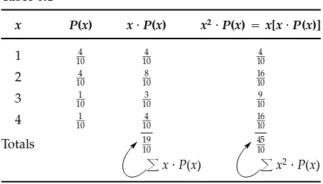
Table 6.1
( ) ( ) ( ) [ ( )]
4 10 4 10 1 10 1 10
4 4 4
10 10 10
4 8 16
10 10 10
1 3 9
10 10 10
1 4 16
10 10 10
19 45
10 10
2
4
4 4 `
4 ` 4
4 4
x P x P P
x
4
EXAMPLE 6.8
Solution
EXAMPLE 6.9
x P x
x P x x P x? x2?P x x x P x?
? ?
^ ^
For the random variable of Example 6.7 (number of girls in a one-child family), calculate the variance and standard deviation using the alternative formula.
We saw in Example 6.7 that . Hence
[ ( )] 0 (0) 1 (1) ( )
(0) ( ) (1) ( ) ( )
Sometimes it is helpful to organize our computations in the form of a table. This is especially recommended if there are more than, say, four or five values for . We illustrate how such a table is used in the following example.
Consider the following probability distribution:
We will use Table 6.1 to find the mean, variance, and standard deviation. 1
2
2 2 2 2 2 1 2
2
1 1 1 1
2 2 4 4
1 1 4 2
!
^
x P x x P x
1 2 3 4
1 2 3 4
Totals
( ) ( )
? 2 ? ? 2
? ? 2
m
s m
8
( )
4 4 4
4 4 4 4
4
4 4
4
4
4 4
4
x P x .
x P x . . . .
. .
x
x
x expected value
E x
E x x P x
x
x
x x
x Remark
Expected value
Definition
EXAMPLE 6.10
Solution
Expected Value
x P x
2
( ) 1 9
[ ( )] (1 9) 4 5 3 61 89
89 94
Note that the mean of the distribution in Example 6.9 is 1.9. This is different from the mean of the individual values (1, 2, 3, 4), which is 2.5. Occasionally, the mean of the distribution is the same as the mean of the individual values. One example is when the distribution is symmetric. (See the distribution discussed at the beginning of this section.)
is just another name for the mean of a random variable. Using this name for the mean is often helpful, because many problems are stated in terms of expectation when the mean is involved. For example, an insurance company might be interested in its expected earnings per customer. This is really just the average.
For a random variable , we define the of the
random variable, denoted by ( ), to be the mean of the random variable. Therefore, for a discrete random variable,
( ) ( )
An insurance company sells a life insurance policy with a face value of $1000 and a yearly premium of $20. If .1% of the policyholders can be expected to die in the course of a year, what would be the company’s expected earnings per policyholder in any year?
Let the amount of money earned by the company from an arbitrary (randomly selected) policyholder in a year. If the policyholder survives the year, then $20. If the policyholder dies, the company must pay out $1000. This minus the $20 premium means that the company loses $980. In other words, on this policyholder the company earns $980 (i.e., $980). The probability that the policyholder dies (i.e., 980) is .001. So the probability that the policyholder lives (i.e.,
20) is .999. Therefore, the probability distribution is
The expected earnings per policyholder are 19
10
2 2 2 45 2
10 !
^
^
^
20 .999 980 .001 ?
? 2 2 2
?
2 2
2
m
s m
s
†
p
( ) 4
4 `
4 4
4
4
4 4
4 4 `
4 ` 4
4
E x x P x
. .
. .
x
. .
expected daily winnings, E x
E x x P x . .
. . .
. .
For a discussion of this and other casino games, see Koshy, T., Santa Monica, Calif.: Goodyear, 1979, Section 4.2. This application was given by John Allen Paulos in
New York: Vintage Books, 1990, p. 47. The same problem is discussed for various sample sizes by Richard J. Larsen and Morris L. Marx in
Englewood Cliffs, N.J.: Prentice-Hall, 1986, p. 158.
Finite Mathematics and Calculus with Applications,
Innumeracy—Mathematical Illiteracy and Its Conse-quences,
Introduction to Mathematical Statistics and Its Applications,
EXAMPLE 6.11 (THE NUMBERS GAME )
Solution
EXAMPLE 6.12
x P x
p
2
( ) ( )
(20)( 999) ( 980)( 001)
19 98 98 19
The company can expect to earn $19 per policyholder (on the average).
This game consists of selecting a three-digit number. If you guess the right number, you are paid $700 for each dollar you bet. Each day there is a new winning number. If a person bets $1 each day for 1 year, how much money can he expect to win (or lose)?
Let the amount won on a given day. If the correct number is guessed, then he wins $700 $1 $699. (Do not forget that it costs $1 to bet.) Otherwise, he loses, so his winnings in this case would be $1. There are 1000 possible three-digit numbers: 000 to 999. The probability of winning (selecting the correct three digits) is 001. The probability of losing is 999. The probability distribution is
Now we find the ( ):
( ) ( ) ( 1)( 999) (699)( 001)
999 699 $ 30
Thus he can expect to lose 30 cents per day (on the average). For the year, he can expect to lose ( 30)(365) $109 50.
A clinic tests blood for a disease that occurs in 1% of the population. The blood samples arrive in batches of 50. The clinic director wondered whether a portion of the blood from each vial should be taken and one test performed on the pooled samples. Then if the test were negative, all samples would be negative. If the test were positive, then each sample would be tested to see which were positive. Under
1 999
1000 1000
^
^
†
1 .999 699 .001
?
2 2
2
2
? 2
( )
For the probability distributions in Exercises 6.22–6.25, find (a) the mean, (b) the variance, and (c) the standard deviation. Also, (d) describe each of the distributions as skewed to the left, skewed to the right, or symmetric. (To organize your computations, it may help to use a table like Table 6.1.)
6.22 6.23 6.24 6.25
( ) ( ) ( ) ( )
6.26
50
50
1 4 1 1
10 10 8 4
1
2 3 3
4
10 10 8
1
3 2 3
4
10 10 8
1
4 1 1
4
10 10 8
4
4 4
4
4 4 `
4 ` 4
x
x x
, x
,
and and and
.
. x
E x x P x . .
. . .
Solution
EXERCISES
x P x
x P x x P x x P x x P x
2
this procedure, what is the expected number of tests that will be performed?
Let number of tests. If all 50 people are free of the disease, only one test will be performed ( 1). If the pooled samples test positive, another 50 tests will be done, so 51. So
1 if all 50 people are negative 51 if at least one person is positive
Since 1% of the population has the disease, 99% do not. So the probability that one person will be negative (does not have the disease) is .99. The probability that all 50 people are negative is the probability that
(first is negative) (second is negative) . . . (50th is negative) Using the Multiplication Rule for Independent Events, the probability of this is ( 99) . At least one person being positive is the opposite (or complement) of all being negative. Hence the probability that at least one person is positive is 1 ( 99) . The probability distribution for is
The expected number of tests is
( ) ( ) (1)( 99) (51)[1 ( 99) ]
605006 20 144691 20 749697
So by pooling the samples, we expect only about 21 tests to be performed on average as opposed to 50 tests if each sample were to be tested.
50
50
50 50
^
5
. .
x
1 ( 99) 51 1 ( 99)
0 0 0 2
3
1 1 1
4
2 2 2
5
3 3 3
A dentist has determined that the number of patients treated in an hour is described 2
( )
6.27
( )
6.28
(a)
(i) (ii) (b)
6.29
6.30
(a) (b) 6.31
2 15 10 15 2 15 1 15
1 20 2 20 3 20 11 20 3 20
4
4 4
x P x
x P x
x
x
x
P x x , , , , , , , , ,
x
x
x x
by the probability distribution given here. Find (a) the mean, (b) the variance, and (c) the standard deviation.
1 2 3 4
The manager of a baseball team has determined that the number of walks issued in a game by one of the pitchers is described by the probability distribution given here. Find (a) the mean, (b) the variance, and (c) the standard deviation.
0 1 2 3 4
Appendix Table A describes how to select random numbers from Appendix Table B.1, a table of random numbers. Let a randomly selected single digit.
Assume that the probability distribution of is as follows:
1
( ) for 0 1 2 3 4 5 6 7 8 9 10
Find the mean of .
Find the standard deviation of .
Randomly select 25 digits from Appendix Table B.1. Calculate the sample mean and the sample standard deviation. Compare these sample results with the population mean and standard deviation in part (a).
An altered die has one dot on one face, two dots on three faces, and three dots on two faces. The die is to be tossed once. Let be the number of dots on the upturned face. Find the mean and variance of .
A card is to be selected from an ordinary deck of 52 cards. Suppose that a casino will pay $10 if you select an ace. If you fail to select an ace, you are required to pay the casino $1.
6.5
THE BINOMIAL PROBABILITY DISTRIBUTION
. . .
6.32
6.33
6.34
Number of Matches Number of Possibilities
1 2000
2 3
2000 2000
O E
O E
trial.
EOE
OOO, EOO, OEO, OOE, OEE, EOE, EEO, EEE
4
binomial experiment.
h j
Consider the experiment of rolling a single die and recording whether the number (of dots) on the top face is odd ( ) or even ( ). This experiment has two possible outcomes: or . We can construct a new experiment by performing this basic experiment over and over a certain number of times. (In a situation like this, the basic experiment is called a ) For example, suppose that we perform this basic experiment three times. If we observed an even number, then an odd, and then an even, we would represent this outcome by . The sample space for the new experiment is
This experiment consisted of repeating a trial a certain number of times; each trial had two possible outcomes. Such an experiment is called a
There are many practical situations that are in essence binomial experiments. For example, we may interview 10,000 voters to see how many favor candidate A.
h j
Hint:
, , , , , ,
S
n S , , S
the original value. If the outcome is a 7, the player loses. If it is the original value, the player wins. The probability that a player will win is .493. Suppose that a player pays $5 to a casino if he loses and is paid $4 for a win. What is the expected loss for the player if he plays (a) one game? (b) ten games?
A bus company is interested in two potential contracts, one for an express and the other for local stops. The probabilities that the bids will be accepted are .70 and .50 with costs of $500 and $750, respectively. The estimated total incomes are $6000 and $10,000, respectively. If the company were allowed only one bid, which bid should they enter?
A high school class decides to raise some money by conducting a raffle. The students plan to sell 2000 tickets at $1 apiece. They will give one prize of $100, two prizes of $50, and three prizes of $25. If you plan to purchase one ticket, what are your expected net winnings? ( The probability of getting the $100 ticket is , of getting a $50 ticket is , and of getting a $25 ticket is .)
In Exercises 5.16 and 5.56, we considered Megabucks, a lottery game conducted by the Massachusetts State Lottery Commission. Megabucks consists of selecting six numbers from the 42 numbers 1 2 3 4 41 42 (no repetitions and order does not matter). The commission selects by chance the six winning numbers. You pay $1 to play. You get a free ticket if three of your numbers match three of the winning numbers, $75 for matching four numbers, $1500 for matching five numbers. Assume you get $1,000,000 if you match all six numbers. The sample space consists of all possible six-number combinations that can be selected. It can be shown that ( ) 5 245 786. The number of elements in that match 0, 1, 2, 3, 4, 5, or 6 winning numbers is given here. What are your expected winnings?
0 1,947,792
1 2,261,952
2 883,575
3 142,800
4 9,450
5 216
. . .
4 4
` 4 4
4
4 4
4 4 4 4
4 4
4
4 4 4 4
4 4
4
4 4
4 4 4
binomial experiment
n trial.
S F
P S p P F q
p q q p p q
binomial random variable x
n x , , , , n
x binomial probability distribution.
O E x
P x
O E E S E
F O
p P S q P F
OOO, EOO, OEO, OOE, OEE, EOE, EEO, EEE
x x
x OOO P P OOO x
EOO, OEO, OOE
P P EOO, OEO, OOE
x OEE, EOE, EEO
P P OEE, EOE, EEO
x EEE P P EEE
Definition
1.
2.
3.
EXAMPLE 6.13
Solution
Here the trial is to interview a voter. This trial has two possible outcomes: Voter favors candidate A or does not favor candidate A. The trial is repeated 10,000 times. As another example, a manufacturer of transistors may select 1000 transistors, then repeatedly perform the trial of checking each transistor to see whether it is defective.
We summarize these ideas in the following definition.
A is an experiment that has the following
properties:
It consists of performing some basic experiment a fixed number of times, . Each time the basic experiment is performed, we call this a
Each trial is identical and has two possible outcomes. We arbitrarily call one outcome success ( ) and the other failure ( ). We call the probability of success ( ) and the probability of failure ( ) . Note that 1. (So 1 .) The values of and do not change from one trial to another.
The trials are independent of one another, that is, the outcome of one trial has no bearing on the outcome of any other trial.
The random variable of interest, the , is the number
of successes in trials. Note that can assume the values 0 1 2 . The probability distribution of is called a
Consider the binomial experiment of rolling a die three times. Each time we record whether the number of dots showing is odd ( ) or even ( ). Let the total number of evens recorded. Find the binomial probability distribution ( ).
The trial is to roll the die and record or . We will call a success. So and failure . Since half the numbers on a die are even and half are odd,
( ) and ( ) . We have seen that the sample space is
Each outcome is equally likely and therefore has the probability . The binomial random variable is the number of successes the number of evens. We must have 0, 1, 2, or 3.
Now 0 corresponds to , so (0) ( ) . The value 1
corresponds to the event . So
(1) ( )
The value 2 corresponds to the event . Therefore,
(2) ( )
Finally, the value 3 corresponds to , so that (3) ( ) . The
binomial probability distribution for this situation is summarized as follows:
1 1
2 2
1 8
1 8 3 8
3 8
1 8
h j
h j
h j
h j
h j
. . .
p
( )
1 8 3 8 3 8 1 8
4
4 4
n p
x
P x
n
p q
q p x n
n
P x p q x , , , , n
x n x
n n
If you have read Sections 5.4 and 5.6, it is not difficult to see why this formula works. First, consider the event consisting of success on the first trials and failure on the next trials:
trials
The trials are independent. Hence the Multiplication Rule for independent events tells us the probability of this is
Now there are a number of different arrangements that can result in successes and failures, all having the same probability, . To count how many ways this can happen, just calculate how many ways we can specify which trials out of the trials are the successes. In Section 5.6, we saw that this number is
! !( )!
So there are this many ways of getting successes and failures, all having probability . Hence, the probability of successes in trials is
! ( )
!( )!
2
2
2
2
2
2
x n x
SS S FF F n
p p p q q q p q
x n x
p q
x n
n C
x n x
x n x p q
x n
n
P x p q
x n x
x P x
p
Y
2
? ? ? ? ? ? ? ?
2
2 2
? ? 2
The essential mathematical ingredients of a binomial experiment are the number of trials , the probability of success on an individual trial , and the number of successes . It would be convenient if we had a formula for the binomial distribution, that is, a formula for ( ), using these mathematical ingredients. Such a formula does exist.
Given a binomial experiment consisting of trials where the probability of success on an individual trial is and the probability of failure is (where 1 ), it can be shown that the probability of exactly successes in trials is given by the following formula :
!
( ) for 0 1 2
!( )!
The symbol ! (read “ factorial”) is defined for any positive integer to be
x n x
x n x
x n x
x n x
n x
x n x
x n x
0 1 2 3
x n x2
2
? ? 2
4
4
4
. . . .
. . . 4 4 4 4 4 4 4 ` 4 4
` 4 ` `
4 4 4
4 4 4 4 4 4
4
4 4 4
4
4 4 4
4 4 4
4 4 4
4 4 4
n n
P x
binomial P x x
p q n
P x x , ,
p q p pq q
P x
n E
O p P E q P O p x
P x x x P x x x P P P P `
binomial probability distribution.
EXAMPLE 6.14
Solution
! 1 2 3
Therefore
3! 1 2 3 6
5! 1 2 3 4 5 120
1! 1 We will agree that 0! 1.
The values of ( ) constitute the The word
is used because the values of ( ) for the various values of are precisely the terms in the binomial expansion of ( ) . For example, when 2, the values of ( ) for 0 1 and 2 are the three terms on the right-hand side of the equation
( ) 2
In Figure 6.3, we display probability histograms for two binomial probability distributions.
Verify that the formula for ( ) in the preceding box does give the probability distribution for the binomial variable of Example 6.13.
For this experiment, 3. Also, success record even ( ) and failure record
odd ( ). Thus ( ) and ( ) 1 . Finally, number of
evens recorded in three rolls of the die. Therefore, 3! ( ) ( ) ( ) !(3 )! Observe that ( ) ( ) ( ) ( ) and so 3! ( ) !(3 )! Now 3! 6 (0)
0!(3 0)! (1) (6)
3! 6
(1)
1!(3 1)! (1) (2)
3! 6
(2)
2!(3 2)! (2) (1)
3! 6
(3)
3!(3 3)! (6) (1)
These results agree with the results of Example 6.13.
2 2 2
1 1
2 2
3 1 1 2 2
3 3 3
1 1 1 1 1
2 2 2 2 8
1 8
1 1 1
8 8 8
1 1 3
8 8 8
1 1 3
8 8 8
1 1 1
8 8 8
n
x x
x x x x
4 4 4
4 4
4 4 4
4
4
4
4 4
4
4 4
4 4 4 `
4 `
4
4
4 4
4 4
4 4 4 `
4 ` 4
P S p .
P F q p .
n x
P x . .
x x
P . .
. . . .
.
P x or x
P x or x P P
. P
P . .
. .
.
P . .
P x or x P P
. . .
A no
EXAMPLE 6.15
(a) (b) (c) Solution (a)
(b)
(c)
Assume that when a certain hunter shoots at a pheasant, the probability of hitting it is .6. Find the probability that the hunter
Will hit exactly four of the next five pheasants at which he shoots. Will hit at least four of the next five.
Will hit at least one of the next five.
trial shoots at a pheasant success hits the pheasant
failure does not hit the pheasant
( ) 6
( ) 1 4
The trial is repeated five times, so 5. The binomial distribution giving the probability of exactly successes in five trials is
5!
( ) ( 6) ( 4)
!(5 )!
The probability of hitting exactly four of the next five pheasants is 5!
(4) ( 6) ( 4)
4!(5 4)! 1 2 3 4 5
( 6) ( 4) (5) ( 6) ( 4) (1 2 3 4) (1)
25920
Now the probability that he hits at least four of the next five pheasants is ( 4 5). But we know that
( 4 5) (4) (5)
25920 (5) and
5!
(5) ( 6) ( 4)
5!(5 5)! 5!
( 6) ( 4) 5!0!
Keeping in mind that 0! 1 and ( 4) 1, we get (5) ( 6) 07776 Thus
( 4 5) (4) (5)
25920 07776 33696
Now we find the probability that he hits at least one out of the next five pheasants. Call the event consisting of hits in the next five shots.
5
4 5 4
4 4
5 5 5
5 0
0 5
x 2x
2
2
2
? ? 2
? ? 2
? ? ? ?
? ? ? ?
? ? ? ?
? ? 2
` 4
4 4 4
4
4 4
4
4 4 4
4
4 4 4
4 4
4
4 4
`
4 4
4 4
4 4 4
A
P A P A
P P A P A P
P
P . .
. .
.
P P
. .
P x
n P x
n x n
P x n
P x n p . x
n n
x x
p p .
x p .
P
P S p
. n x
P x EXAMPLE 6.16
Solution
Then the complement of this event, , consists of hitting at least one. Since ( ) ( ) 1, we have
(hitting at least 1) ( ) 1 ( ) 1 (0) Now we need only evaluate (0) and subtract from 1:
5!
(0) ( 6) ( 4)
0!(5 0)! 5!
(1) ( 4) ( 4) 5!
01024 Therefore,
(hitting at least one) 1 (0)
1 01024
98976
The formula for calculating binomial probabilities ( ) can be rather unpleasant to use for all but very small values of . Appendix Table B.2 gives values of ( ) for various values of and up to 25. [In Chapter 7, we develop a method of finding ( ) for values of 25.]
Let’s use Appendix Table B.2 to find ( ) when 5, 60, and 4. In Example 6.15, we found this value to be .259 rounded to three decimal places. In the far left column, locate the desired value of , in this case 5. To the right and below this, locate the row containing the desired value of , here 4. At the top of the table, locate the column containing the desired value of , here 60. Now where the row containing 4 and the column containing 60 intersect, we find the value of (4), namely, .259. (See Table 6.2, which shows a portion of Appendix Table B.2.)
Notice that some of the probabilities in Appendix Table B.2 are represented as 0 . This means that the probability is so small as to be negligible and hence may be assigned the value 0 in calculations.
Thirty percent of the voters in a large voting district are veterans. If 10 voters are randomly selected, find the probability that less than five will be veterans.
This is a binomial experiment. trial select voter success voter is a veteran
( ) proportion of voters in district who are veterans 30
10 (repeat the trial 10 times) number of veterans
We want to find ( 5). Using Appendix Table B.2, we get 0 5 0
5 5
2
2 2
? ? 2
? ?
2 2
.
. . .
4 ` ` ` `
4 ` ` ` `
4
4 4
4 4
4 4
4 ` ` ` `
4 ` `
4
4
P x P P P P P
. . . . .
.
Note: p
P S p .
n x
P x P x x
P x P P P P
. .
.
x x EXAMPLE 6.17
Solution
( 5) (0) (1) (2) (3) (4)
028 121 233 267 200
849
Since the voting district is large, we can safely assume that the value of remains essentially the same from one trial to the next.
A company that manufactures color television sets claims that only 5% of its sets will need to be adjusted by a technician before being sold. If an appliance dealer sells 20 of these sets, how likely is it that more than three of them will need to be adjusted?
trial check one of the sets success it needs adjustment
( ) 05
20 (repeat the trial 20 times)
number out of 20 that need adjustment
We want to find ( 3). Using Appendix Table B.2, add the values of ( ) for from 4 to 20:
( 3) (4) (5) (19) (20)
013 002 (negligible terms) 015
We conclude that if the manufacturer is right, it is very unlikely that more than three sets will need to be adjusted.
Example 6.17 provides some insight into how the binomial distribution might be used in statistical inference. For example, the manager of an appliance store chain received a large shipment of these TV sets, and she wished to test the manufacturer’s claim that only 5% (or perhaps less) will need adjustment. She might randomly select 20 sets from the shipment and determine how many of these sets need adjustment. We can view the population as consisting of the entire shipment of TV sets from the manufacturer. The 20 sets then constitute a sample from the population. Based on the number of TV sets out of the 20 that are in need of adjustment, she will decide whether there is strong evidence to suggest that more than 5% of the sets in the population will be in need of adjustment. She would want the evidence to be strong because if she concludes that more than 5% of the population need adjusting, she will return the entire shipment—a drastic step. What criterion might she use? That is, if the number of TV sets out of the 20 needing adjustment, how large should be for the manager to conclude that the shipment should be returned?
Since the manufacturer claims 5% (or less) will need adjusting, it would not be alarming if we found 5% of the 20, or one TV set, needing adjusting. Perhaps two sets would not even be alarming. (After all, we can expect some fluctuation from one
,
.
4 4
4
4 4 4
4 4 4
4 4
x
x
x
x
the proportion of elements in a population possessing a certain characteristic of interest may be viewed as the probability of success in a binomial experiment.
P S p .
n
p . x
x
E x n p
n p
x
E x n p
population proportions,
for a binomial experiment
Mean and Variance of a Binomial Random Variable
batch of 20 sets to the next.) But the larger the value of , the more we are inclined to believe that more than 5% of the population will need adjusting. If the value of is large enough (relative to 1), the manager would reject the manufacturer’s claim (and the shipment as well). By “large enough” we mean so large that it would be highly unlikely that we would observe such a large value of if the manufacturer’s claim were true. Note that we have already seen a range of such unlikely values in Example 6.17. We said that it would be very unlikely (only a 1.5% chance) that we would get a value of greater than 3 if in fact the manufacturer were correct. Therefore, the manager could use this as her criterion: If more than three of the TV sets do need adjusting, the evidence would strongly suggest that the manufacturer’s claim should be rejected.
We will see in later chapters that a binomial experiment is a very important concept in a variety of statistical inference problems ranging from industrial quality control to voter preference studies. The reason for this is that
In Example 6.16, we discussed the proportion of voters in a district who were veterans. This proportion was .30. A trial consisted of selecting a voter by chance. A success occurs if the voter selected is a veteran. The binomial experiment consisted of performing the trial 10 times. Since 30% of the voters are veterans, the probability that a voter selected on a single trial will be a veteran is .30. This is the probability of success, so that ( ) 30. Sometimes such proportions are unknown, and we can use a binomial variable to study these proportions. We investigate these proportions, known as
in Chapter 9.
Suppose that we consider the binomial experiment of tossing a fair coin 100 times. Let success heads. Clearly, 5. Let the number of heads. When the coin is tossed 100 times, how many heads would you expect to get, that is, what is your best guess? We would guess that half (or 50) would be heads. In other words, the expected value of is 50. This can be obtained from the formula
( ) 100 ( ) 50
This formula, in fact, works in general. That is, it can be proved rigorously, using the formula for given previously in this chapter, that
consisting of trials with the probability of success , the mean or expected value of is
( )
It can also be proved, using the formula for variance given previously in the chapter, that for a binomial variable
1 2
? ?
?
m
6.35
(a) (b) (c)
(d)
(e)
6.36
(a) (b) (c)
6.37
(a) (b) (c)
6.38
(a) (b) (c) (d) (e) 6.39
(a) (b) (c) (d) (e) 6.40
(a) (b) (c)
4
4 4 4
4 4
n p q
n p q
4 4 4
4 4 4
4 4 4
4 4 4
4 4 4
4 4 4
EXERCISES
Thus, for the number of heads when a coin is tossed 100 times (100)( )( ) 25
25 5
2
2 1 1
2 2 !
n p . x P x
x x x
n p . x P x
x x x
n p . x
x x x x x
n p . x
x x x x x
Which of the following are binomial experiments? For those that are not, indicate which part of the definition of a binomial experiment does not apply.
Tossing a fair coin 1000 times and counting the number of times a head appears Tossing a fair coin and counting the number of tosses before a head appears Checking five students for drug use from a class of 30 students in which 10% use drugs
A state agency randomly selects 20 liquor stores, with replacement, and counts the number of stores involved in price fixing
A shipment of 40 appliances contains two defectives. A dealer tests 15 of the appliances and counts the number that fail to meet specifications.
Consider a binomial experiment with 4, 6, and the number of successes. Use the formula for ( ) to find the probability that
0 1 2
Consider a binomial experiment with 5, 7, and the number of successes. Use the formula for ( ) to find the probability that
3 4 5
Consider a binomial experiment with 11, 4, and the number of successes. Use Appendix Table B.2 to find the probability that
is less than 2.
is greater than 5 and less than 8.
is greater than or equal to 5 and less than or equal to 8. equals 6.
is greater than 0.
Consider a binomial experiment with 9, 7, and the number of successes. Use Appendix Table B.2 to find the probability that
is less than 3. equals 3.
is greater than 3 and less than 5.
is greater than or equal to 3 and less than or equal to 5. is less than 9.
Sixty percent of the voters in a large town are opposed to a proposed development. If 20 voters are selected at random, find the probability that
10 are opposed to the proposed development.
More than 13 are opposed to the proposed development. Less than 10 are opposed to the proposed development.
? ?
? ?
s
s
6.41
(a) (b) (c) 6.42
(a) (b) 6.43
(a) (b) 6.44
6.45
6.46
(a) (b)
6.47
(a) (b) (c)
6.48
(a) (b) (c)
(d) 6.49
(a) (b)
Source: The 1994 Information Please Almanac,
Forty percent of the student body at a large university are in favor of a ban on drinking in the dormitories. Suppose 15 students are to be randomly selected. Find the probability that
Seven favor the ban.
Fewer than four favor the ban. More than two favor the ban.
It has been reported that 30% of the population of women who had given birth in the last year and had less than a high school education were in the labor force (
1994, p. 843). In a random sample of 25 from this population, find the probability that
Ten are in the labor force.
The sample will contain 4, 5, 6, or 7 women in the labor force.
Sixty percent of the Framingham Heart Study participants have a total serum choles-terol level below 238. An HMO statistician is interested in interviewing 15 people. If 15 people are randomly selected, find the probability that
Eight people will have a total serum cholesterol level below 238. Five people or more will have a total serum cholesterol level below 238. A retailer decides that he will reject a large shipment of light bulbs if there is more than one defective bulb in a sample of size 10. If the defective rate is .10, what is the probability that the retailer will reject the shipment?
A person has a 5% chance of winning a free ticket in a state lottery. If she plays the game 25 times, what is the probability she will win one or more free tickets?
Five percent of the cans of handballs purchased at a sporting goods store are unac-ceptable. If 12 cans are purchased, find the probability that
All of the cans are acceptable. More than two cans are unacceptable.
Suppose 200 cans were bought. What is the expected number of unacceptable cans? A screening examination is required of all applicants for a technical writing position. The examination consists of 16 questions. Each question has five choices, consisting of the correct answer and four incorrect answers. A curious applicant wonders about some probabilities if she were to randomly guess at each question.
What is the probability of getting three correct? What is the probability of getting two or more correct?
If 50 applicants took the exam and each guessed randomly at all the questions, what would you guess the mean number of correct answers to be?
Thirty-eight percent of the people have blood type A. In a random sample of 20 people, find the probability that
One will have type A. Two or three will have type A. One or more will not have type A.
Suppose 100 samples of size 20 were selected, and the number of people in each sample with type A was recorded.
What should be the approximate mean number of people with type A? Ten percent of the people have blood type B. In a random sample of 20 people, find the probability that
Three will have type B.
6.6
USING MINITAB (OPTIONAL)
(c)(d) 6.50
6.51
(a) (b) (c)
(d)
(e)
6.52
6.53 (a) (b) 6.54
6.55
4 4 4
4 4
4 4 4
4 4 4
PDF Command
The PDF (probability distribution function) command can be used to find
prob-x
x
plus
Castenada Partida,
Statistics and the Law,
x
x n
p . p . p . p .
p .
n n
n p . p .
Fewer than two will have type B.
Suppose 100 samples of size 20 were selected, and the number of people in each sample with type B was recorded.
What should be the approximate mean number of people with type B?
There are 4,230,000 eligible voters in a state, of whom 147,000 are black. A sample of 100 voters is to be selected. Let be the number of blacks. Assume a binomial experiment. Find (a) the mean, (b) the variance, and (c) the standard deviation of . Between 1972 and 1974, 15 out of 405 teachers (3.7%) hired in Hazelwood, St. Louis County, Missouri, were black. In St. Louis County the nearby city of St. Louis, 15.4% of teachers were black. The Equal Employment Opportunity Commission (EEOC) sued Hazelwood for discrimination against blacks and won the case in the court of appeals. Assuming that the 405 teachers hired constitute a random sample from a population of teachers, 15.4% of whom are black, answer the following:
What is the mean (or expected) number of black teachers? What is the standard deviation?
In the case of v. 430 U.S. 482 (1977), the “Standard Deviation Rule” was advanced. This states that if the observed value (15 teachers in the Hazelwood case) is more than 2 or 3 standard deviations from the expected value, discrimination may be present. How many standard deviations away from the expected value is the observed value of 15?
On appeal to the Supreme Court, the decision of the court of appeals was vacated. The Supreme Court noted that the relevant job market for teachers might well be St. Louis County alone (which does not include the city of St. Louis), where the percentage of black teachers is 5.7%. Redo parts (a), (b), and (c) using this percentage.
This analysis assumes that the selection of the 405 teachers is a random process (with respect to race). Can the selection of teachers be considered a random process?
For a discussion, see DeGroot, M., S. Fienberg, and J. Kadane, New York: Wiley, 1986, pp. 1–48.
Seven percent of printed circuit boards made by the SKC company are defective. A company official wishes to see whether the percentage of defective boards in a current batch has decreased. A sample of size 50 is to be selected. Let be the number of defectives. Assume a binomial experiment. If there is no change from the 7% figure, find (a) the mean, (b) the variance, and (c) the standard deviation of .
Consider a binomial experiment with 4. Construct probability histograms when 3 and 7. Comment on the relationship between the two.
4 and 6. Comment on the relationship between the two.
Consider a binomial experiment with 5. Construct probability histograms when 3 and 5. Comment on the shapes of the distributions.
© ©
© ©
4 P
5 .6
4
P .
K1
P P
P P
5 .6 C1
P P
Session Commands Dialog Box
Calc Probability Distributions Binomial Number