getdoc827b. 536KB Jun 04 2011 12:04:35 AM

(1)

E l e c t ro n ic

Jo u r n

a l o

f P

r o b

a b i l i t y

Vol. 10 (2005), Paper no. 33, pages 1044-1115. Journal URL

http://www.math.washington.edu/_∼ejpecp/

Dynamic Scheduling of a Parallel Server System

in Heavy Traffic with Complete Resource Pooling:

Asymptotic Optimality of a Threshold Policy

S. L. Bell and R. J. Williams 1 Department of Mathematics University of California, San Diego

La Jolla CA 92093-0112 Email: williams@math.ucsd.edu

http://www.math.ucsd.edu/_∼williams

Abstract

We consider a parallel server queueing system consisting of a bank of buffers for holding incoming jobs and a bank of flexible servers for processing these jobs. Incoming jobs are classified into one of several different classes (or buffers). Jobs within a class are processed on a first-in-first-out basis, where the processing of a given job may be performed by any server from a given (class-dependent) subset of the bank of servers. The random service time of a job may depend on both its class and the server providing the service. Each job departs the system after receiving service from one server. The system manager seeks to minimize holding costs by dynamically scheduling waiting jobs to available servers. We consider a parameter regime in which the system satisfies both a heavy traffic and a complete resource pooling condition. Our cost function is an expected cumulative discounted cost of holding jobs in the system, where the (undiscounted) cost per unit time is a linear function of normalized (with heavy traffic scaling) queue length. In a prior work [42], the second author proposed a continuous review threshold control policy for use in such a parallel server system. This policy was advanced as an “interpretation” of the analytic solution to an associated Brownian control problem (formal heavy traffic diffusion approximation). In this paper we show that the policy proposed in [42] is asymptotically optimal in the heavy traffic limit and that the limiting cost is the same as the optimal cost in the Brownian control problem.

Keywords and phrases: Stochastic networks, dynamic control, resource pooling, heavy traffic, diffusion approximations, Brownian control problems, state space collapse, threshold policies, large deviations.

AMS Subject Classification (2000): Primary 60K25, 68M20, 90B36; secondary 60J70. Submitted to EJP on July 16, 2004. Final version accepted on August 17, 2005.

1_{Research supported in part by NSF Grants DMS-0071408 and DMS-0305272, a John Simon Guggenheim}

(2)

1 Introduction

We consider a dynamic scheduling problem for a parallel server queueing system. This system might be viewed as a model for a manufacturing or computer system, consisting of a bank of buffers for holding incoming jobs and a bank of flexible servers for processing these jobs (see e.g., [23]). Incoming jobs are classified into one of several different classes (or buffers). Jobs within a class are served on a first-in-first-out basis and each job may be served by any server from a given subset of the bank of servers (this subset may depend on the class). In addition, a given server may be able to service more than one class. Jobs depart the system after receiving one service. Jobs of each class incur linear holding costs while present within the system. The system manager seeks to minimize holding costs by dynamically allocating waiting jobs to available servers.

The parallel server system is described in more detail in Section 2 below. With the exception of a few special cases, the dynamic scheduling problem for this system cannot be analyzed exactly and it is natural to consider more tractable approximations. One class of such approximations are the so-called Brownian control problems which were introduced and developed as formal heavy traffic approximations to queueing control problems by Harrison in a series of papers [12, 19, 16, 17]. Various authors (see for example [7, 8, 20, 21, 24, 29, 30, 39]) have used analysis of these Brownian control problems, together with clever interpretation of their optimal (analytic) solutions, to suggest “good” policies for certain queueing control problems. (We note that some authors have used other approximations for queueing control problems such as fluid models, see e.g. [32] and references therein, but here we restrict attention to Brownian control problems as approximations.)

For the parallel server system considered here, Harrison and L´opez [18] studied the associated Brownian control problem and identified a condition under which the solution of that problem exhibitscomplete resource pooling, i.e., in the Brownian model, the efforts of the individual servers can be efficiently combined to act as a single pooled resource or “superserver”. Under this condition, Harrison and L´opez [18] conjectured that a “discrete review” scheduling policy (for the original parallel server system), obtained by using the BIGSTEP discretization procedure of Harrison [14], is asymptotically optimal in the heavy traffic limit. They did not attempt to prove the conjecture, although, in a slightly earlier work, Harrison [15] did prove asymptotic optimality of a discrete review policy for a two server case with special distributional assumptions.

Here, focusing on the parameter regime associated with heavy traffic and complete resource pooling, we first review the formulation and solution of the Brownian control problem. Then we prove that a continuous review “tree-based” threshold policy proposed by the second author in [42] is asymptotically optimal in the heavy traffic limit. (Independently of [42], Squillante et al. [35] proposed a tree-based threshold policy for the parallel server system. However, their policy is in general different from the one described in [42]. An example illustrating this is given in Section 5.4.) Our treatment of the Brownian control problem is similar to that in [18, 42] and our description of the candidate threshold policy is similar to that in [42], although some more details are included here. On the other hand, the proof of asymptotic optimality of this policy is new. In a related work [3], we have already proved that this policy is asymptotically optimal for a particular two-server, two-buffer system. Indeed, techniques developed in [3] have been useful for analysis of the more complex multiserver case treated here. These techniques have also recently been used in part by Budhiraja and Ghosh [7] in treating a classic controlled queueing network example known as the criss-cross network.

(4)

linear holding costs. Although this provides an asymptotically optimal policy for the parallel server problem, we think it is still of interest to establish asymptotic optimality of a simple continuous review threshold policy, as we do here. Indeed, the policy proposed in [1] and the method of proof are substantially different from those used here. The discrete review policy of [1] observes the state of the system at discrete review times and determines open loop controls to be used over the periods between review times. Their control typically changes with the state observed at the beginning of each of these “review periods”. Our policy is a simple threshold priority policy. It continuously monitors the state, but the control only changes when a threshold is crossed or a queue becomes empty. Furthermore, our policy exploits a tree structure of the parallel server system, whereas the policy of [1], which is designed for more general systems with feedback, does not exploit the tree structure when restricted to parallel server systems. Finally, our proof involves an induction procedure to prove estimates related to the tree structure; there is not an analogue of this inductive proof in the paper [1].

The other related works are by Stolyar [36], who considers a generalized switch, which operates in discrete time, and Mandelbaum and Stolyar [31], who consider a parallel server system. Although it does not allow routing, Stolyar’s generalized switch is somewhat more general than a parallel server system operating in discrete time. In particular, it allows service rates that depend on the state of a random environment. Assuming heavy traffic and a resource pooling condition, which is slightly more general than a complete resource pooling condition, Stolyar [36] proves asymptotic optimality of a MaxWeight policy, for holding costs that are positive linear combinations of the individual queue lengths raised to the power β+ 1 where β >0. In particular, the holding costs are not linear in the queue length. An advantage of the MaxWeight policy (which exploits the non-linear nature of the holding cost function) is that it does not require knowledge of the arrival rates for its execution, although checking the heavy traffic and resource pooling conditions does involve these rates.

Following on from [36], in [31], Mandelbaum and Stolyar focus on a parallel server system (operating in continuous time). Assuming heavy traffic and complete resource pooling conditions they prove asymptotic optimality of a MaxWeight policy (called a generalized cµ-rule there), for holding costs that are sums of strictly increasing, strictly convex functions of the individual queue lengths. (They also prove a related result where queue lengths are replaced by sojourn times.) Again, the nonlinear nature of the holding cost function allows the authors to specify a policy that does not require knowledge of the arrival rates (nor of a solution of a certain dual linear program). Although Mandelbaum and Stolyar [31] conjecture a policy for linear holding costs (which like ours makes use of the solution of a dual linear program), they stop short of proving asymptotic optimality of that policy.

Thus, assuming heavy traffic scaling, the current paper provides the only proof of asymptotic optimality of a continuous review policy for the parallel server system with linear holding costs under a complete resource pooling condition. An additional difference between our work and that in [1, 31, 36] is that we impose finite exponential moment assumptions on our primitive stochastic processes, whereas only finite moment assumptions (of order 2 +ǫ) are needed for the results in [1, 31, 36]. We conjecture that our exponential moment assumptions could be relaxed to moment conditions of sufficiently high order, at the expense of an increase in the size of our (logarithmic) thresholds. We have not pursued this conjecture here, having chosen the tradeoff of smaller thresholds at the expense of exponential moment assumptions.

This paper is organized as follows. In Section 2, we describe the model of a parallel server system considered here. In Section 3 we introduce a sequence of such systems, indexed byr(where

(5)

queue length (in diffusion scale). In Section 3, we also review the notion of heavy traffic defined in [16, 18] using a linear program, and recall its interpretation in terms of the behavior of an associated fluid model, as previously described in [42]. In Section 4, we describe the Brownian control problem associated with the sequence of parallel server systems, and, under the complete resource pooling condition of Harrison and L´opez [18], we review the solution of the Brownian control problem obtained in [18] using a reduced form of the problem called the equivalent workload formulation [16, 19]. The complete resource pooling condition ensures that the Brownian workload process is one-dimensional. Moreover, from [18] we know that this condition is equivalent to uniqueness of a solution to the dual to the linear program described in Section 3. In Section 5, we describe the dynamic threshold policy proposed in [42] for use in the parallel server system. This policy exploits a tree structure of a graph containing the servers and buffers as nodes. We then state the main result (Theorem 5.4) which implies that this policy is asymptotically optimal in the heavy traffic limit and that the limiting cost is the same as the optimal cost in the Brownian control problem. An outline of our method of proof is given in Section 6. The details of the proof are contained in Sections 7–9. Here a critical role is played by our analysis in Section 7 of what we call the residual processes, which measure the deviations of the queue lengths from the threshold levels, or from zero if a queue does not have a threshold on it, when the threshold policy is used. This allows us to establish a form of “state space collapse” (see Theorems 6.1 and 5.3) under this policy. The techniques used in proving state space collapse build on and extend those introduced in [3]. In particular, a major new feature is the need to show that allocations of time to various activities stay close to their nominal allocations over sufficiently long time intervals (with high probability), which in turn is used to show that the residual processes stay close to zero (with high probability). Using a suitable numbering of the buffers, the proof of state space collapse proceeds by induction on the buffer number, highlighting the fact that the queue length for a particular buffer depends (via the threshold policy) on the queue lengths associated with lower numbered buffers. Another new aspect of our proof lies in Section 9, where a certain uniform integrability is used to prove convergence of normalized cost functions associated with the sequence of parallel server systems, operating under the threshold policy, to the optimal cost function for the Brownian control problem. To establish the uniform integrability, estimates of the probabilities that the residual processes deviate far from zero need to be sufficiently precise (cf. Theorem 7.7). This accounts for the appearance of the polynomial terms in (I)–(III) of Section 7.2. Also, in the proof of the uniform integrability of the normalized idletime processes, a technical point that was overlooked in the proof of the analogous result in [3] is corrected. Specifically, the proof is divided into two separate cases depending on the size of the time index (cf. (9.34)–(9.36)). (In the proof of Theorem 5.3 in [3], the estimates in (173) and (176) should have been divided into two cases corresponding tor2t >2/˜ǫand r2t≤2/˜ǫ.)

1.1 Notation and Terminology

The set of non-negative integers will be denoted by IN and the value +_∞ will simply be denoted by _∞. For any real number x,_⌊x_⌋ will denote the integer part of x, i.e., the greatest integer that is less than or equal to x, and ⌈x⌉ will denote the smallest integer that is greater than or equal to x. We let IR+ denote [0,∞). The m-dimensional (m≥ 1) Euclidean space will be denoted by IRm _{and IR}m

+ will denote them-dimensional positive orthant, [0,∞)m. Let| · | denote the norm on IRm given by |x|= Pm

i=1|xi| for x ∈ IRm. We define a sum over an empty index set to be zero. Vectors in IRmshould be treated as column vectors unless indicated otherwise, inequalities between vectors should be interpreted componentwise, the transpose of a vectorawill be denoted bya′_{, the}

diagonal matrix with the entries of a vector aon its diagonal will be denoted by diag(a), and the dot product of two vectors aand b in IRm will be denoted by a_·b. For any set _S, let _|S| denote the cardinality of _S.

(6)

domain IR+. That is, Dm _{is the set of all functions} _ω _{: IR+} _→ _IRm _{that are right continuous on}

IR+ and have finite left limits on (0,∞). The member of Dm that stays at the origin in IRm for all time will be denoted by 0. Forω _∈Dm _and _t_≥_{0, let}

kω_kt= sup s∈[0,t]|

ω(s)_|. (1.1)

Consider Dm _{to be endowed with the usual Skorokhod J}

1-topology (see [10]). LetMm denote the Borel σ-algebra on Dm _{associated with the J}

1-topology. All of the continuous-time processes in this paper will be assumed to have sample paths in Dm _{for some}_m_≥_{1. (We shall frequently use}

the term process in place of stochastic process.) Suppose _{Wn_}∞

n=1 is a sequence of processes with sample paths in Dm for some m ≥1. Then we say that _{Wn_}∞

n=1 is tight if and only if the probability measures induced by the Wn’s on (Dm_,_Mm_{) form a tight sequence, i.e., they form a weakly relatively compact sequence in the space}

of probability measures on (Dm_,_Mm_{). The notation “}_Wn _⇒ _W_{”, where} _W _{is a process with}

sample paths in Dm_{, will mean that the probability measures induced by the}_Wn_{’s on (D}m_,_Mm₎

converge weakly to the probability measure on (Dm_,_Mm_{) induced by}_W_{. If for each}_n_,_Wn_and_W

are defined on the same probability space, we say that Wn _{converges to}_W _{uniformly on compact}

time intervals in probability (u.o.c. in prob.), ifP(_kWn₋_W_k

t≥ε)→0 as n→ ∞for each ε >0

and t ≥0. We note that if {Wn_} _{is a sequence of processes and} _W _{is a continuous deterministic}

process (all defined on the same probability space) thenWn_⇒_W _{is equivalent to}_Wn_→_W _u.o.c.

in prob. This is implicitly used several times in the proofs below to combine statements involving convergence in distribution to deterministic processes.

2 Parallel Server System

2.1 System Structure

Our parallel server system consists of I infinite capacity buffers for holding jobs awaiting service, indexed by i ∈ I ≡ {1, . . . ,I}, and K (non-identical) servers working in parallel, indexed by

k _{∈ K ≡ {}1, . . . ,K_}. Each buffer has its own stream of jobs arriving from outside the system. Arrivals to bufferiare called classijobs and jobs are ordered within each buffer according to their arrival times, with the earliest arrival being at the head of the line. Each entering job requires a single service before it exits the system. Several different servers may be capable of processing (or serving) a particular job class. Service of a given job class i by a given server k is called a processing activity. We assume that there are J≤ I·K possible processing activities labeled by

j_{∈ J ≡ {}1, . . . ,J_}. The correspondences between activities and classes, and activities and servers, are described by two deterministic matricesC,A, whereCis anI_×Jmatrix with

Cij =

(

1 if activityj processes classi,

0 otherwise, (2.1)

and Ais a K×Jmatrix with

Akj =

(

1 if server kperforms activity j,

0 otherwise. (2.2)

(7)

capable of being processed by at least one activity and each server is capable of performing at least one activity).

Once a job has commenced service at a server, it remains there until its service is complete, even if its service is interrupted for some time (e.g., by preemption by a job of another class). A server may not start on a new job of class i until it has finished serving any classi job that it is working on or that is in suspension at the server. In addition, a server cannot work unless it has a job to work on. When taking a new job from a buffer, a server always takes the job at the head of the line. (For concreteness, we suppose that a deterministic tie-breaking rule is used when two (or more) servers want to simultaneously take jobs from the same buffer, e.g., there is an ordering of the servers and lower numbered servers take jobs before higher numbered ones.) This setup allows a job to be allocated to a server just before it begins service, rather than upon arrival to the system. We assume that the system is initially empty.

2.2 Stochastic Primitives

All random variables and stochastic processes used in our model description are assumed to be defined on a given complete probability space (Ω,F,P). The expectation operator under P will be denoted byE. Fori_{∈ I}, we take as given a sequence of strictly positive i.i.d. random variables {ui(ℓ), ℓ= 1,2, . . .} with mean λ−i 1 ∈(0,∞) and squared coefficient of variation (variance divided

by the square of the mean) a2_i ∈ [0,∞). We interpret ui(ℓ) as the interarrival time between the (ℓ₋1)st _{and the} _ℓth _{arrival to class} _i _{where, by convention, the “0}th _{arrival” is assumed to occur} at time zero. Settingξi(0) = 0 and

ξi(n) =

n

X

ℓ=1

ui(ℓ), n= 1,2, . . . , (2.3)

we define

Ai(t) = sup{n≥0 :ξi(n)≤t} for allt≥0. (2.4) Then Ai(t) is the number of arrivals to class i that have occurred in [0, t], and λi is the long

run arrival rate to class i. For j ∈ J, we take as given a sequence of strictly positive i.i.d. random variables _{vj(ℓ), ℓ= 1,2, . . ._} with mean µ−_j1_∈(0,_∞) and squared coefficient of variation

b2_j _∈[0,_∞). We interpretvj(ℓ) as the amount of service time required by the ℓth job processed by activityj, and µj as the long run rate at which activity j could process its associated class of jobs

i(j) if the associated server k(j) worked continuously and exclusively on this class. For j∈ J, let

ηj(0) = 0,

ηj(n) = n

X

ℓ=1

vj(ℓ), n= 1,2, . . . , (2.5)

and

Sj(t) = sup{n≥0 :ηj(n)≤t} for all t≥0. (2.6)

Then Sj(t) is the number of jobs that activity j could process in [0, t] if the associated server worked continuously and exclusively on the associated class of jobs during this time interval. The interarrival time sequences _{ui(ℓ), ℓ = 1,2, . . .}, i ∈ I, and service time sequences {vj(ℓ), ℓ =

1,2, . . .},j∈ J, are all assumed to be mutually independent.

2.3 Scheduling Control and Performance Measures

Scheduling control is exerted by specifying a J-dimensional allocation process T = _{T(t), t _≥ 0_} where

(8)

and Tj(t) is the cumulative amount of service time devoted to activity j ∈ J by the associated serverk(j) in the time interval [0, t]. NowT must satisfy certain properties that go along with its interpretation. Indeed, one could give a discrete-event type description of the properties that T

must have, including any system specific constraints such as no preemption of service. However, for our analysis, we shall only need the properties ofT described in (2.11)–(2.16) below.

Let

I(t) =1t−AT(t), t≥0, (2.8)

where 1 is the K-dimensional vector of all ones. Then for each k∈ K, Ik(t) is interpreted as the cumulative amount of time that server k has been idle up to time t. A natural constraint onT is that each component of the cumulative idletime processI must be continuous and non-decreasing. Since each column of the matrixAcontains the number one exactly once, this immediately implies that each component ofT is Lipschitz continuous with a Lipschitz constant of one. For eachj_{∈ J},

Sj(Tj(t)) is interpreted as the number of complete jobs processed by activityj in [0, t]. Fori∈ I,

let

Qi(t) =Ai(t)− J

X

j=1

CijSj(Tj(t)), t≥0, (2.9)

which we write in vector form (with a slight abuse of notation forS(T(t))) as

Q(t) =A(t)₋CS(T(t)), t_≥0. (2.10) Then Qi(t) is interpreted as the number of class i jobs that are either in queue or “in progress” (i.e., being served or in suspension) at timet. We regardQandI as performance measures for our system.

We shall use the following minimal set of properties of any scheduling controlT with associated queue length process Qand idletime process I. For all i_{∈ I},j_{∈ J},k_{∈ K},

Tj(t)_{∈ F} for each t_≥0, (2.11)

Tj is Lipschitz continuous with a Lipschitz constant of one, (2.12)

Tj is non-decreasing, andTj(0) = 0,

Ik is continuous, non-decreasing, andIk(0) = 0, (2.13)

Qi(t)≥0 for all t≥0. (2.14)

Properties (2.12) and (2.13) are for each sample path. For later reference, we collect here the queueing system equations satisfied by Qand I:

Q(t) = A(t)₋CS(T(t)), t_≥0, (2.15)

I(t) = 1t₋AT(t), t_≥0, (2.16)

where Q,T and I satisfy properties (2.11)–(2.14). We emphasize that these are descriptive equa-tions satisfied by the queueing system, given C, A, A, S and a control T, which suffice for the purposes of our analysis. In particular, we do not intend them to be a complete, discrete-event type description of the dynamics.

(9)

The cost function we shall use involves linear holding costs associated with the expense of holding jobs of each class in the system until they have completed service. We defer the precise description of this cost function to the next section, since it is formulated in terms of normalized queue lengths, where the normalization is in diffusion scale. Indeed, in the next section, we describe the sequence of parallel server systems to be used in formulating the notion of heavy traffic asymptotic optimality.

3 Sequence of Systems, Heavy Traffic, and the Cost Function

For the parallel server system described in the last section, the problem of finding a control policy that minimizes a cost associated with holding jobs in the system is notoriously difficult. One possible means for discriminating between policies is to look for policies that outperform others in some asymptotic regime. Here we regard the parallel server system as a member of a sequence of systems indexed by r that is approaching heavy traffic (this notion is defined below). In this asymptotic regime, the queue length process is normalized with diffusive scaling – this corresponds to viewing the system over long intervals of time of order r2 (where r will tend to infinity in the asymptotic limit) and regarding a single job as only having a small contribution to the overall cost of storage, where this is quantified to be of order 1/r. The setup in this section is a generalization of that used in [3].

3.1 Sequence of Systems and Large Deviation Assumptions

Consider a sequence of parallel server systems indexed by r, where r tends to infinity through a sequence of values in [1,_∞). These systems all have the same basic structure as that described in Section 2, except that the arrival and service rates, scheduling control, and form of the cost function (which is defined below in Section 3.3) are allowed to depend on r. Accordingly, we shall indicate the dependence of relevant parameters and processes onr by appending a superscript to them. We assume that the interarrival and service times are given for eachr _≥1,i_{∈ I},j _{∈ J}, by

ur_i(ℓ) = 1

λr i

ˇ

ui(ℓ), vr_j(ℓ) = 1

µr j

ˇ

vj(ℓ), forℓ= 1,2, . . . , (3.1)

where the ˇui(ℓ), ˇvj(ℓ), do not depend on r, have mean one and squared coefficients of variation

a2_i,b2_j, respectively. The sequences _{uiˇ (ℓ), ℓ= 1,2, . . ._}, _{ˇvj(ℓ), ℓ= 1,2, . . ._}, i_{∈ I}, j _{∈ J} are all mutually independent sequences of i.i.d. random variables. (The above structure is a convenient means of allowing the sequence of systems to approach heavy traffic by simply changing arrival and service rates while keeping the underlying sources of variability ˇui(ℓ), ˇvj(ℓ) fixed. This type of setup has been used previously by others in treating heavy traffic limits, see e.g., Peterson [34]. For a first reading, the reader may like to simply chooseλr ₌_λ_and _µr₌_µ _{for all}_r_{. Indeed, that}

simplification is made in the paper [42].)

We make the following assumption on the first order parameters associated with our sequence of systems.

Assumption 3.1 There are vectors λ_∈IRI

+, µ∈IR

J

+, such that (i) λi >0 for alli_{∈ I}, µj >0 for all j_{∈ J},

(ii) λr_→_λ, _µr _→_µ, _as _r _{→ ∞}_.

In addition, we make the following exponential moment assumptions to ensure that certainlarge deviation estimates hold for the renewal processesAr

i,i∈ I, andSjr, j ∈ J (cf. Lemma 6.7 below

(10)

Assumption 3.2 For i∈ I, j∈ J, and all ℓ≥1, let

ui(ℓ) =

1

λiuˇi(ℓ), vj(ℓ) =

1

µjˇvj(ℓ). (3.2)

Assume that there is a non-empty open neighborhood O0 of 0∈IR such that for all l∈ O0,

Λai(l) ≡ logE[elui(1)]<∞, for all i∈ I, and (3.3)

Λs_j(l) _≡ logE[elvj(1)_]_<_∞_, _{for all} _j_{∈ J}_. _(3.4)

Note that (3.3) and (3.4) hold with ℓ in place of 1 for all ℓ= 1,2, . . ., since{ui(ℓ), ℓ = 1,2, . . .},

i_{∈ I}, and _{vj(ℓ), ℓ= 1,2, . . ._},j _{∈ J}, are each sequences of i.i.d. random variables.

Remark. This finiteness of exponential moments assumption allows us to prove asymptotic opti-mality of a threshold policy with thresholds of order logr. We conjecture that this condition could be relaxed to a sufficiently high finite moment assumption, and our method of proof would still work, provided larger thresholds are used to allow for larger deviations of the primitive renewal processes from their rate processes. Here we have chosen the tradeoff of smaller thresholds and exponential moment assumptions, rather than larger thresholds and certain finite moment assump-tions. We note that to adapt our proof to use finite moment assumptions, Lemma 6.7 would need to be modified to use estimates of the primitive renewal processes based on sufficiently high finite moments, rather than exponential moments (cf. [1, 5, 31, 36]). In addition, this lemma is used repeatedly in proving the main theoretical estimates embodied in Theorem 7.7. The latter is proved by induction and the proof involves a recursive increase in the size of the thresholds as well as an increase in the size of the error probability which involves powers of r2t. Thus, in order to deter-mine the necessary order of a finite moment condition and the size of accompanying thresholds, one would need to carefully examine this recursive proof.

3.2 Heavy Traffic and Fluid Model

There is no conventional notion of heavy traffic for our model, since the nominal (or average) load on a server depends on the scheduling policy. Harrison [16] (see also Laws [29] and Harrison and Van Mieghem [19]) has proposed a notion of heavy traffic for stochastic networks with scheduling control. For our sequence of parallel server systems, Harrison’s condition is the same as Assumption 3.3 below. Here, and henceforth, we define

R=Cdiag(µ).

Assumption 3.3 There is a unique optimal solution (ρ∗_{, x}∗_,₎ _{of the linear program:}

minimize ρ subject to Rx=λ, Ax_≤ρ1 and x_≥0. (3.5) Moreover, that solution is such thatρ∗ = 1 and Ax∗ =1.

Remark. It will turn out that under Assumption 3.3,x∗

j is the average fraction of time that server k(j) should devote to activityj. For this reason,x∗ is called the nominal allocation vector.

(11)

A fluid model solution (with zero initial condition) is a triple of continuous (deterministic) functions ( ¯Q,T ,¯ I¯) defined on [0,_∞), where ¯Qtakes values in IRI

, ¯T takes values in IRJ

and ¯I takes values in IRK

, such that

¯

Q(t) = λt₋RT¯(t), t_≥0, (3.6) ¯

I(t) = 1t₋AT¯(t), t_≥0, (3.7) and for all i,j,k,

¯

Tj is Lipschitz continuous with a Lipschitz constant of one,

it is non-decreasing, and ¯Tj(0) = 0, (3.8)

¯

Ik is continuous, non-decreasing, and ¯Ik(0) = 0, (3.9)

¯

Qi(t)_≥0 for all t_≥0. (3.10)

A continuous function ¯T : [0,∞)→IRJ such that (3.8)–(3.10) hold for ¯Q,I¯defined by (3.6)–(3.7) will be called afluid control. For a given fluid control ¯T, we say the fluid system is balanced if the associated fluid “queue length” ¯Q does not change with time (cf. Harrison [13]). Here, since the system starts empty, that means ¯Q ≡ 0. In addition, we say the fluid system incurs no idleness (or all fluid servers are fully occupied) if ¯I _≡0, i.e.,AT¯(t) =1t for allt_≥0.

Definition 3.4 The fluid model is in heavy traffic if the following two conditions hold: (i) there is a unique fluid control T¯∗ under which the fluid system is balanced, and (ii) under T¯∗, the fluid system incurs no idleness.

Since any fluid control is differentiable at almost every time (by (3.8)), we can convert the above notion of heavy traffic into one involving the ratesx∗(t) = ˙¯T∗(t), where “ ˙ ” denotes time derivative. This leads to the following lemma which is stated and proved in [42] (cf. Lemma 3.3 there).

Lemma 3.5 The fluid model is in heavy traffic if and only if Assumption 3.3 holds.

We impose the following heavy traffic assumption on our sequence of parallel server systems, henceforth.

Assumption 3.6 (Heavy Traffic) For the sequence of parallel server systems defined in Section 3.1 and satisfying Assumptions 3.1 and 3.2, assume that Assumption 3.3 holds and that there is a vector θ_∈IRI

such that

r(λr−Rrx∗)→θ, as r → ∞, (3.11)

where Rr ₌_C_diag(_µr_).

For the formulation of the Brownian control problem, it will be helpful to distinguish basic activities j which have a strictly positive nominal fluid allocation levelx∗_j fromnon-basic activities

j for which x∗

j = 0. By relabeling the activities if necessary, we may and do assume henceforth

(12)

3.3 Diffusion Scaling and the Cost Function

For a fixed r and scheduling control Tr_{, the associated queue length process} _Qr _{= (}_Qr

1, . . . , QrI)′

and idletime processIr _{= (}_Ir

1, . . . IKr)′ are given by (2.15)–(2.16) where the superscript r needs to

be appended toA,S,Q,I and T there. The diffusion scaled queue length process ˆQr_{and idletime}

process ˆIr _{are defined by}

ˆ

Qr(t) =r−1Qr(r2t), Iˆr(t) =r−1Ir(r2t), t_≥0. (3.12) We consider an expected cumulative discounted holding cost for the diffusion scaled queue length process and control Tr_:

ˆ

Jr(Tr) =E µZ ∞

0

e−γth_·Qˆr(t)dt

¶

, (3.13)

where γ > 0 is a fixed constant (discount factor) and h = (h1, . . . , hI)′, hi >0 for all i ∈ I, is a

constant vector of holding costs per unit time per unit of diffusion scaled queue length. Recall that “ _·” denotes the dot product between two vectors.

To write equations for ˆQr_,_I_ˆr_{, we introduce centered and diffusion scaled versions ˆ}_Ar_,_S_ˆr _{of the}

primitive processes Ar_,_Sr_:

ˆ

Ar(t) =r−1¡

Ar(r2t)−λrr2t¢

, Sˆr(t) =r−1¡

Sr(r2t)−µrr2t¢

, (3.14)

a deviation process Yˆr _{(which measures normalized deviations of server time allocations from the}

nominal allocations given byx∗_):

ˆ

Yr(t) =r−1¡

x∗r2t₋Tr(r2t)¢

, (3.15)

and a fluid scaled allocation process ¯Tr_:

¯

Tr(t) =r−2Tr(r2t). (3.16) On substituting the above into (2.15)–(2.16), we obtain

ˆ

Qr(t) = Aˆr(t)₋CSˆr( ¯Tr(t)) +r(λr₋Rrx∗)t+RrYˆr(t), (3.17) ˆ

Ir(t) = AYˆr(t), (3.18)

where by (2.12)–(2.14) we have ˆ

Ir

k is continuous, non-decreasing and ˆIkr(0) = 0, for all k∈ K, (3.19)

ˆ

Qr_i(t)_≥0 for all t_≥0 and i_{∈ I}. (3.20)

On combining Assumption 3.1 with the finite variance and mutual independence of the stochas-tic primitive sequences of i.i.d. random variables _{uˇi(ℓ)}∞ℓ=1, i ∈ I, {ˇvj(ℓ)}∞ℓ=1, j ∈ J, we may deduce from renewal process functional central limit theorems (cf. [22]) that

( Âr,Sˆr)_⇒( Ã,S˜), asr _{→ ∞}, (3.21) where Ã, ˜S are independent, Ã is an I-dimensional driftless Brownian motion that starts from the origin and has a diagonal covariance matrix whose ith _{diagonal entry is} _λ

ia2i, and ˜S is a

(13)

4 Brownian Control Problem

4.1 Formulation

Under the heavy traffic assumption of the previous section, to keep queue lengths from growing on average, it seems desirable to choose a control policy for the sequence of parallel server systems that asymptotically on average allocates service to the processing activities in accordance with the proportions given by x∗. To see how to achieve this and to do so in an optimal manner, following a method proposed by Harrison [12, 15, 18], we consider the following Brownian control problem which is a formal diffusion approximation to control problems for the sequence of parallel server systems. The relationship between the Brownian model and the fluid model is analogous to the relationship between the central limit theorem and the law of large numbers.

Definition 4.1 (Brownian control problem) minimize E

µZ ∞

0

e−γth·Q˜(t)dt

¶

(4.1)

using a J-dimensional control process Y˜ = ( ˜Y1, . . . ,YJ˜ )′ such that ˜

Q(t) = ˜X(t) +RY˜(t) for allt_≥0, (4.2) ˜

I(t) =AY˜(t) for allt_≥0, (4.3) ˜

Ik is non-decreasing and I˜k(0)≥0, for allk∈ K, (4.4)

˜

Yj is non-increasing and Yj˜ (0)_≤0, for j=B+1, . . . ,J, (4.5) ˜

Qi(t)≥0 for allt≥0, i∈ I, (4.6) where X˜ is an I-dimensional Brownian motion that starts from the origin, has drift θ (cf. (3.11)) and a diagonal covariance matrix whose ith _{diagonal entry is equal to} _λi_a2

i+

PJ

j=1Cij µjb2_jx∗_j for i_{∈ I}.

The above Brownian control problem is a slight variant of that used by Harrison and L´opez [18]. In particular, we allow ˜Y to anticipate the future of ˜X. The process ˜X is the formal limit in distribution of ˆXr_{, where for}_t_≥_0,

ˆ

Xr(t)≡Aˆr(t)−CSˆr( ¯Tr(t)) +r(λr−Rrx∗)t. (4.7) The control process ˜Y in the Brownian control problem is a formal limit of the deviation processes

ˆ

Yr_{. (cf. (3.15)). The non-increasing assumption in property (4.5) corresponds to the fact that}

ˆ

Yr

j(t) = −r−1Tjr(r2t) is non-increasing whenever j is a non-basic activity. The initial conditions

on ˜I and ˜Yj, j = B+ 1, . . . ,J, in (4.4)–(4.5) are relaxed from those in the prelimit to allow for the possibility of an initial jump in the queue length in the Brownian control problem. (In fact, for the optimal solution of the Brownian control problem, under the complete resource pooling condition to be assumed later, such a jump will not occur and then the Brownian control problem is equivalent to one in which ˜I(0) = 0, ˜Y(0) = 0.)

4.2 Solution via Workload Assuming Complete Resource Pooling

For open processing networks, of which parallel server systems are a special case, Harrison and Van Mieghem [19] showed that the Brownian control problem can be reduced to an equivalent formula-tion involving a typically lower dimensional state process. In this reducformula-tion, the Brownian analogue

˜

(14)

called the workload dimension and the reduced form of the Brownian control problem is called an equivalent workload formulation. Intuitively, the reduction in [19] is achieved by ignoring certain “reversible directions” in which the process ˜Q can be controlled to move instantaneously without incurring any idleness and without using any non-basic activities; in addition, such movements are instantaneously reversible. In a work [16] following on from [19], Harrison elaborated on an interpretation of the reversible displacements and proposed a “canonical” choice for the workload matrixM, which reduces the possibilities forM to a finite set. This choice uses extremal optimal solutions to the dual to the linear program used to define heavy traffic, cf. (3.5). For the parallel server situation considered here, that dual program has the following form.

Dual Program

maximize y_·λ subject to y′R_≤z′A, z_·1_≤1 and z_≥0. (4.8) We shall focus on the case in which the workload dimension is one. This is equivalent to there being a unique optimal solution of the dual program (4.8). Indeed, for parallel server systems, The-orem 4.3 below gives several conditions that are equivalent to this assumption of a one-dimensional workload process. For the statement of this result, we need the following notion of communicating servers.

Definition 4.2 Consider the graphG in which servers and buffers form the nodes and (undirected) edges between nodes are given by basic activities. We say that all servers communicate via basic activities if, for each pair of servers, there is a path in _G joining all of the servers.

Theorem 4.3 The following conditions are equivalent (for parallel server systems). (i) the workload dimension L is one,

(ii) the dual program (4.8) has a unique optimal solution (y∗_{, z}∗_),

(iii) the number of basic activities B is equal to I+K₋1, (iv) all servers communicate via basic activities,

(v) the graph _G is a tree.

Proof. The equivalence of the first four statements of the theorem was derived in Harrison and L´opez [18], and the equivalence of these statements with (v) was noted in [42]. Also, as noted by Ata and Kumar [1], the equivalence of (i) with (iii) can also be seen by observing from Corollary 6.2 in Bramson and Williams [6] that since the matrix A has exactly one positive entry in each column, the workload dimensionL=I+K₋B,whereB is the number of basic activities. ✷

Henceforth we make the following assumption.

Assumption 4.4 (Complete Resource Pooling) The equivalent conditions (i)–(v) of Theorem 4.3 hold.

The intuition behind the term “complete resource pooling” is that, under this condition, all servers can communicate via basic activities, and it is reasonable to conjecture that the efforts of the servers (or resources) can be combined in a cooperative manner so that they act effectively as a single pooled resource. A main aim of this work is to show that this intuition is correct.

Let (y∗_{, z}∗_{) be the unique optimal solution of (4.8). By complementary slackness, ((}_y∗₎′_R)

j

= ((z∗)′A)j for j = 1, . . .B. Let u∗ be the (J−B)-dimensional vector of dual “slack variables”

defined by ((y∗₎′_R₋₍_z∗₎′_A)

(15)

Lemma 4.5 We have y∗ >0, z∗ >0, u∗>0,

(y∗)′R= (z∗)′A₋[0′ (u∗)′], and z∗_·1= 1, (4.9) where 1 is the K-dimensional vector of ones, 0′ _{is a} _{B-dimensional row vector of zeros.}

Proof. This is proved in [18] (Corollary to Proposition 3) using the relation between the primal and dual linear programs. ✷

Now, we review a solution of the Brownian control problem obtained by Harrison and L´opez [18]. This exploits the fact that the workload is one-dimensional.

For ˜Q satisfying (4.2)–(4.6), define ˜W = y∗ ·Q˜, which Harrison [16] calls the (Brownian) workload. Let ˜YN be the (J−B)-dimensional process whose components are ˜Yj,j=B+ 1, . . . ,J.

By Lemma 4.5 and (4.2)–(4.6), ˜

W(t) =y∗_·X˜(t) + ˜V(t) for allt_≥0, (4.10) where

˜

V ≡z∗·I˜−u∗·YN˜ is non-decreasing and ˜V(0)≥0, (4.11) ˜

W(t)≥0 for allt≥0. (4.12)

Now, for each t_≥0, since the holding cost vector h >0 andy∗ _>_{0, we have}

h·Q˜(t) =

I

X

i=1 µ

hi y∗

i

¶

y_i∗Qi˜ (t)≥h∗W˜(t) (4.13)

where

h∗ ≡

I

min

i=1 µ

hi y∗

i

¶

. (4.14)

It is well-known and straightforward to see that any solution pair ( ˜W ,V˜) of (4.10)–(4.12) must satisfy for all t≥0,

˜

V(t)_≥V˜∗(t)_≡ sup 0≤s≤t

³

−y∗_·X˜(s)´, (4.15)

and hence ˜W(t)≥W˜∗(t) where ˜

W∗(t) = y∗·X˜(t) + ˜V∗(t). (4.16) The process ˜W∗ _{is a one-dimensional} _{reflected Brownian motion} _{driven by the one-dimensional}

Brownian motion y∗·X˜, and ˜V∗ is its local time at zero (see e.g., [9], Chapter 8). In particular, ˜

V∗ can have a point of increase at timet only if ˜W∗(t) = 0. Now, let i∗ _{be a class index such that} _h∗ ₌_h

i∗/y∗

i∗, i.e., the minimum in (4.14) is achieved at

i=i∗, and letk∗ be a server that can serve classi∗ via a basic activity. Note that neitheri∗ nork∗

need be unique in general. Then the following choices ˜Q∗ and ˜I∗ for ˜Qand ˜I ensure that for each

t _≥ 0, properties (4.4)–(4.6) hold and the inequality in (4.13) is an equality with ˜W(t) = ˜W∗₍_t₎

there:

˜

Q∗_i∗(t) = ˜W∗(t)/y_i∗∗, Q˜∗_i(t) = 0 for alli6=i∗, (4.17) ˜

(16)

A control process ˜Y∗ such that (4.2)–(4.6) hold with ˜Q∗,Y˜∗,I˜∗ in place of ˜Q,Y ,˜ I˜there is given in [42]. It can be readily verified that this is an optimal solution for the Brownian control problem (cf. [18]) and the associated minimum cost is

J∗_≡E

µZ ∞

0

e−γth_·Q˜∗(t)dt

¶

=h∗E µZ ∞

0

e−γtW˜∗(t)dt

¶

. (4.19)

The quantityJ∗ is finite and can be computed as in Section 5.3 of [11].

Now, even though the Brownian control problem can be analyzed exactly (as above), the solution obtained does not automatically translate to a policy for the sequence of parallel server systems. However, some desirable features are suggested by the form of (4.17)–(4.18), namely, (a) try to keep the bulk of the work in the class i∗ _{with the lowest (or equal lowest) ratio of holding cost to}

workload contribution, i.e., the class i with the lowest value of hi/yi∗, (b) try to ensure that the

bulk of the idleness is incurred only when there is almost no work in the entire system, and (c) try to ensure that the bulk of the idletime is incurred by serverk∗ _alone.

4.3 Approaches to Interpreting the Solution

Harrison [14] has proposed a general scheme (called BIGSTEP) for obtaining candidate policies for a queueing control problem from a solution of the associated Brownian control problem. The policies obtained in this manner are so-called discrete-review policies which allow review of the system status and changes in the control rule only at a fixed discrete set of times. For a two-server example (with Poisson arrivals, deterministic service times and particular values forλ, µ), a discrete-review policy was constructed and shown to be asymptotically optimal in Harrison [15]. Based on their solution of the Brownian control problem and the general scheme laid out by Harrison [14], Harrison and L´opez [18] proposed the use of a discrete review policy for the multiserver problem considered here, but they did not prove asymptotic optimality of this policy. Recently, Ata and Kumar [1] have proved asymptotic optimality of a discrete review policy for open stochastic processing networks that include parallel server systems, under heavy traffic and complete resource pooling conditions. Another approach to translation of solutions of Brownian control problems into viable policies has been proposed by Kushner et al. (see e.g., [25, 26, 27]). However this also involves discretization by way of numerical approximation. We note that, of the works by Kushner et al. mentioned above, the paper by Kushner and Chen [25] is the closest to the current one in that it considers a parallel server model. However, it is in a very different parameter regime, namely one that corresponds to heavy traffic but withno resource pooling.

(17)

5 Threshold Policy and Main Results

In this section, we describe a dynamic threshold policy for our sequence of parallel server systems and state our main results, which imply that this policy is asymptotically optimal. Recall that we are assuming throughout that the heavy traffic (Assumption 3.6) and complete resource pooling (Assumption 4.4) conditions hold. The threshold policy takes advantage of the tree structure of the server-buffer treeG. In reviewing our description of the policy, the reader may find it helpful to refer to the examples in [42], where a version of this policy was first described. We also include two additional examples here in Section 5.4 to help explain the policy. We note that there can be many asymptotically optimal policies. The one described here is simply proposed as one that is intuitively appealing and that is asymptotically optimal.

Independently of [42], Squillante et al. [35] proposed a tree-based threshold priority policy for a parallel server system. However, their policy is different from the one described here. The second example we give in Section 5.4 is used to illustrate this.

5.1 Tree Conventions

The threshold policy only involves the use of basic activities (and so in the following description of the policy, the word “activity” will be synonymous with “basic activity”). Also, the terms class and buffer will be used interchangeably. A key to the description of the policy is a hierarchical structure of the server-buffer tree _G and an associated protocol for the dynamic allocation of (preemptive-resume) class priorities at each server. This protocol is described in an iterative manner, working from the bottom of the tree up towards the root. (One should imagine a tree as growing downwards from its root and the root as being at the highest level.) A server tree _S, which results from suppressing the buffers in G, will be helpful for describing the iterative procedure. Recall the solution of the Brownian control problem described in Section 4.2. The root of the server-buffer tree _G(and of the server tree_S) is taken to be a serverk∗ _{which serves the “cheapest” class}_i∗ _via

a (basic) activity. Classes (or buffers) that link one level of servers to those at the next highest level in the tree_G are called transition classes (or transition buffers).

5.2 Threshold Policy

To describe the threshold policy, we first focus on the server tree S and imagine it arranged in levels with the root k∗ at the highest level of _S. We proceed inductively up through the levels in the tree _S.

First, consider a server at the lowest level. As a server within the server-buffer tree G, this server is to service its classes according to a priority scheme that gives lowest priority to the class that is immediately above the server in _G. The latter class is also served by a server in the next level up in S and so is a transition class. There will always be such a class unless the server is at the root of the tree. On the other hand there may be zero, one or more classes lying below a server at the lowest level in the tree. The relative priority ranking of these classes (if any) is not so important. These are all terminal classes in that there are no servers below them. Here, for concreteness, we rank the classes so that for a given server, the lower numbered classes receive priority over the higher numbered ones. For future use, we place a threshold on the transition class immediately above each server in the lowest level of S.

(18)

classes are served first). However, if the number of jobs in a transition class associated with such an activity is at or below the threshold for that class, service of that activity is suspended. The next priority is given to activities that service (terminal) classes that are only served by that server (again ranked according to a scheme that gives lower numbered classes higher priority), and lowest priority is given to the activity serving the transition class that is immediately above the server in the server-buffer tree. This transition class should again have a threshold placed on it such that service of that class by the server at the next highest level will be suspended when the number of jobs in the class is equal to or below the threshold level. If two or more servers simultaneously begin to serve a particular transition buffer, a tie breaking rule is used to decide which server takes a job first. For concreteness we suppose that the lowest numbered server shall select a job before the next higher numbered server, and so on. Note that two servers in the same level cannot both serve the same buffer below them since_G is a tree.

This process is repeated until the root of the server tree is reached. At the root, the same procedure is applied as for lower server levels, except that there are no activities above the root server in the server-buffer tree and an overriding rule is that lowest priority is given to the “cheapest” classi∗.

The idea behind the threshold policy is to keep servers below the root level busy the bulk of the time (indeed, they should only be rarely idle and their idletimes should vanish on diffusion scale as the heavy traffic limit is approached), while simultaneously preventing the queue lengths of all classes except i∗ from growing appreciably on diffusion scale. Transition buffers are used to achieve these two competing goals. Intuitively, when the queue length for a transition class gets to or below its threshold, any service of that class by the server immediately above it in the tree is suspended and this causes temporary overloading (on average) of the servers below, which prevents these servers from incurring much idleness. When the queue length for the transition class builds up to a level above its threshold, then assistance from the higher server is again permitted and the servers below are temporarily underloaded (on average) and so queue lengths for classes serviced by these servers are prevented from growing too large. The intended effect of this policy is to allow the movement (via the transition buffers) of excess work from lower level to higher level buffers (and eventually, by an upwards cascade, to the buffer for classi∗), while simultaneously keeping all servers busy the bulk of the time, unless the entire system is nearly empty and even then to ensure that the vast majority of the idleness is incurred by the server k∗ _{at the root of the tree.}

5.3 Threshold Sizes

(19)

❄ ❄ ❄ ❄ ❄

1 2 3 4 5

❅ ❅

❅ ❅_❅_{❘ ❄}

¡ ¡ ¡ ¡ ¡

✠ ❄

❅ ❅

❅ ❅ ❘ ❄

❅ ❅

❅ ❅_❅_❘

¡ ¡ ¡ ¡ ✠ ♥

1 2♥ 3♥ 4♥

❄ ❄ ❄ ❄

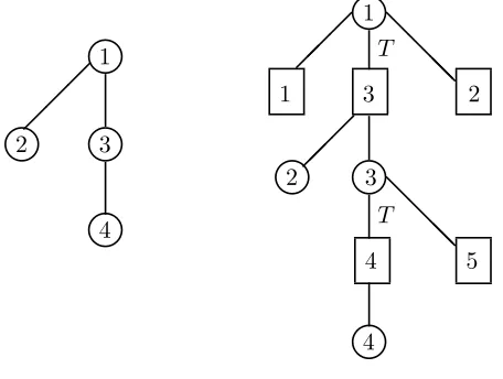
Figure 1: A parallel server system with four servers and five classes. Only basic activities are shown.

♥ 1 ¡ ¡ ¡ ♥

2 3♥

♥ 4

♥ 1 ¡ ¡

¡ T

❅ ❅

❅❅

1 3 2

¡ ¡ ¡ ♥

2 3♥

T

❅ ❅

❅❅ 5 4

♥ 4

Figure 2: The server tree (on the left) and server-buffer tree (on the right) for the system pictured in Figure 1 with i∗ _{= 2 and} _k∗_{= 1. Activities subject to thresholding have a} _T _{beside them.}

5.4 Examples

In this subsection we give two examples to illustrate our threshold policy. The second example is also used to illustrate that our policy differs from that of [35].

Example 5.1 Consider the parallel server system pictured in Figure 1, where only basic activities are shown. Suppose for this that i∗ _{= 2} _{and hence} _k∗ _{= 1. The server tree and server-buffer tree,}

with server 1 as root, are depicted in Figure 2. Activities subject to thresholding have a T beside them.

(20)

λ1 λ2 λ3

❄ ❄ ❄

1 2 3

µ1 µ2 µ3 µ4 µ5

❄ ❄ ❄

¡ ¡ ¡ ¡ ✠

❅ ❅

❅ ❅ ❘

♥ ♥ ♥

1 2 3

❄ ❄ ❄

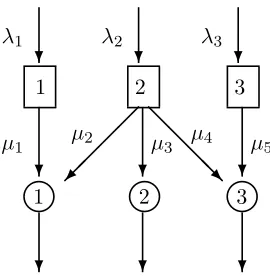
Figure 3: A parallel server system with three servers and three classes (or buffers).

suspends service of a job of class 3whenever the number of jobs in that class reaches or goes below the threshold for the class. In that case, server 1 turns its attention to class 1 jobs until there are no jobs of that class to serve and then finally server 1 turns to serving jobs of the lowest priority class i∗ _{= 2. Whenever the number of jobs in class} ₃ _{again goes above the threshold for that class,}

server 1 switches attention back to serving that class.

The policy proposed by Squillante et al. [35] involves the allocation of priorities for each server based on a local optimization of cµ-type with suspension of certain thresholded activities when the associated class levels are at or below threshold. Their policy locally takes account of the tree structure, whereas our policy exploits the global tree structure. The following example illustrates how the two policies can yield different priority rules.

Example 5.2 Consider the three-server, three-class parallel server system pictured in Figure 3. This example was considered by Squillante et al. [35] with two different sets of parameters in their Examples 4 and 5. For their Example 4 (using our notation), λ = (0.4,1.4,0.6) and µ = (1,0.5,1,0.25,1). Here

C=





1 0 0 0 0 0 1 1 1 0 0 0 0 0 1



, A= 



1 1 0 0 0 0 0 1 0 0 0 0 0 1 1



.

The heavy traffic Assumption 3.3 is readily verified to hold, where x∗ _{= (0}_.₄_,₀_.₆_,₁_,₀_.₄_,₀_._{6), and}

hence all activities are basic. Since B = 5 = I+K−1, it follows from Theorem 4.3 that the complete resource pooling Assumption 4.4 holds. Noting Lemma 4.5, the unique solution of the dual program (4.8) is readily verified to be z∗ ₌ _y∗ _{= (2}_/₇_,₄_/₇_,₁_/_{7). Let} _h _{= (1}_,₁₀₀_,_{10). Then}

(hi/y_i∗, i= 1,2,3) = (7/2,175,70) and soh∗ = 7/2, i∗= 1 andk∗ = 1, since class 1 is only served by server 1.

Under our threshold policy, server 3 gives priority to class3jobs over those of class 2, server2 always serves class2jobs when there are such available, and service of class2 by server1is subject to a threshold in the sense that server 1 gives priority to class 2 except when the number of jobs in class 2 is at or below its threshold and then server 1 suspends service of any class 2 job it is processing and switches attention to serving class 1 jobs until the number of jobs in class 2 once again exceeds the threshold for class 2 (cf. Figure 4).

(21)

♥ 1 ¡ ¡ ¡ ¡ ♥

2 3♥

♥ 1 ¡ ¡

¡ T

1 2

¡ ¡ ¡ ♥

2 3♥

3

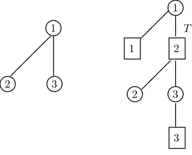
Figure 4: The server tree (on the left) and server-buffer tree (on the right) for the system pictured in Figure 3 with the data described for Example 5.2. The activity subject to thresholding under our policy is indicated with aT.

thresholding, such that if the number of jobs in class2 is above threshold, server3 serves jobs from class 2, whereas when the number of jobs in class 2 is at or below threshold, server 3 serves jobs from class 3.

5.5 Main Results

In Sections 7 and 8, we prove the following limit theorem for a certain sequence of allocation processes _{Tr,∗_}_{. For each} _r_,_Tr,∗ _{is obtained by applying the aforementioned threshold policy in}

the rth parallel server system. The sizes of the thresholds on the transition buffers are of order logr. The specific threshold sizes, which, as mentioned above, increase as one moves across and up the server-buffer tree, are specified precisely in the next section (cf. (6.4)).

Theorem 5.3 Consider the sequence of parallel server systems indexed by r, where therth system operates under the allocation process Tr,∗ _{described above. Then the associated normalized queue}

length and idletime processes satisfy

( ˆQr,Iˆr)_⇒( ˜Q∗,I˜∗), as r_{→ ∞}, (5.1) where Q˜∗

i = 0 for all i ∈ I\{i∗}, I˜k∗ = 0 for all k ∈ K\{k∗}, Q˜∗i∗ is a one-dimensional reflected Brownian motion that starts from the origin and has drift (y∗ ·θ)/y∗_i∗ and variance parameter

PI

i=1(yi∗)2(λia2i +

PJ

j=1Cijµjb2jx∗j)/(yi∗∗)2, and I˜_k∗∗ is a specific multiple of the local time at the origin of Q˜∗

i∗ (In fact, Q˜∗_i∗, I˜_k∗∗ are equivalent in law to the processes given by (4.15)–(4.18)). Recall the definitions ofJ∗and ˆJr_{from (4.19) and (3.13), respectively. The following theorem is the}

main result of this paper. It is proved in Section 9 using Theorem 5.3. It shows thatJ∗ is the best that one can achieve asymptotically and that this asymptotically minimal cost is achieved by the sequence of dynamic controls{Tr,∗}. Thus we conclude that our threshold policy is asymptotically optimal.

Theorem 5.4 (Asymptotic Optimality) Suppose that {Tr_} _{is any sequence of scheduling controls}

(one for each member of the sequence of parallel server systems). Then lim inf

r→∞

ˆ

Jr(Tr)_≥J∗ = lim

r→∞

ˆ

Jr(Tr,∗), (5.2)

(22)

Remark. Note that our threshold policy prescribes that a threshold be placed on class i∗ if that class is a transition class. We conjecture that the policy which removes the threshold in this case is also asymptotically optimal, but we keep the threshold here as a means to simplify our proof. In particular, servers below i∗ may experience significant idletime if the threshold is removed. Our threshold policy also involves preemption of service. There is a corresponding policy without preemption that we conjecture has the same behavior in the heavy traffic limit, since in that regime a maximum ofJjobs (in suspension or not) should not impact the asymptotic behavior of the system.

6 Preliminaries and Outline of the Proof

In this section, we will precisely specify the threshold sizes used for _{Tr,∗_}_{, give some preliminary}

definitions and results, and outline the proofs of Theorems 5.3 and 5.4. Details of the proofs are contained in Sections 7–9.

Recall from Section 2 that _I,_K, and _J index job classes, servers, and activities, respectively. Basic Activities Convention. Since our threshold policy only uses basic activities, to simplify notation, in this section and the next (Sections 6 and 7) only, the index set J will just include the basic activities1,2, . . . ,B. With this convention, Jwill be synonymous with B.

6.1 The Server-Buffer Tree G: Layers and Buffer Renumbering

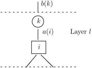
To facilitate our proof, we refine our description of the server-buffer tree,G. We say that the server-buffer tree consists of one or more layers, where a layer consists of a server level along with the buffer level immediately below it. (At the lowest layer, the buffer level may be empty.) Activities that serve the buffers (from above and below) in a particular layer are also considered part of that same layer. We denote the number of layers byl∗ and enumerate the layers in increasing order as one moves up the tree, so that layer 1 is the lowest layer and layerl∗ _{is the top layer, consisting of}

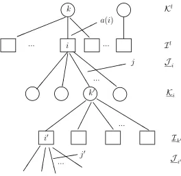
server k∗, the buffers served by this server (including buffer i∗), and the corresponding activities. Assumingl >1, Figure 5 depicts layers l andl₋1 in a server-buffer tree.

For each layerl= 1, . . . , l∗_{, we denote the collection of servers in layer}_l_by_Kl _{and the collection}

of buffers in layerlbyIl_{. For}_k_{∈ K}l_{, the collection of buffers in layer}_l_{served by server}_k_{is denoted}

by _I_k (in Figure 5, i _{∈ I}_k). The activity that serves buffer i _{∈ I}_k using server k is labeled a(i) (“a” is mnemonic for “above”), the collection of activities that serve bufferifrom below is denoted by Ji, and the collection of servers in layer l−1 that serve buffer i using the activities in Ji is

denoted by _K_i (the underscores indicate that the quantities are “below”). We let _Ji denote the

collection of all activities that service buffer i, i.e., activity a(i) together with _J_i. Note that for each bufferi∈ I1_,_J

i =∅,Ki=∅, i.e., layer 1 does not contain any activities that serve buffers in

this layer from below. In fact, we may even have_I1=_∅.

Without loss of generality, we assume the following left-to-right arrangement and renumbering convention for buffers in the server-buffer tree G. This simplifies the description of the priorities associated with our threshold policy. (The simplest way to think of doing the arrangement is to work from the top of the tree downwards.)

Arrangement Convention. Fork∈ K\{k∗}, the buffers inIkare arranged so that the transition

buffers are positioned to the left of the non-transition buffers, and within the groups of transition and non-transition buffers, the lower numbered buffers are to the left of the higher numbered ones. For k = k∗_{, the arrangement in the previous sentence holds with the exception that buffer} _i∗ _is

placed at the far right in level Il∗

=Ik∗.

(23)

✒✑

Figure 5: Layers land l−1 of a server-buffer tree.

to the right is buffer _|I1_|. Continuing with layer 2, the buffer farthest to the left is labeled_|I1_|+ 1, and the one farthest to the right is labeled _|I1_|₊_|I2_|_{, and so on ending with layer} _l∗_{. If} _I1 ₌_∅_, we use the same scheme except that buffer 1 will then be the buffer farthest to the left in layer 2.

Under the arrangement and renumbering conventions, for any serverk, all of the buffers served bykare numbered such that lower priority buffers have higher numbers. (This is true whether the buffers are above or below the server and whether they are transition or non-transition buffers.) In particular, for k ₆= k∗, the higher priority transition buffers in _I_k are numbered lower than the non-transition buffers in _I_k and the transition buffer above khas a higher number than all of the buffers in Ik. If k = k∗, the same statement holds with the exception that i∗ is the highest

numbered buffer and has the lowest priority among all buffers in _I_k∗. It also follows from our numbering scheme that i∗₌_I.

Figure 6 illustrates the server-buffer graph of Figure 2, first with the arrangement convention imposed and then with the renumbering convention applied, where the correspondence between the old and new numbering of classes (or buffers) is given by 1_→4′_,₂_→₅′_,₃_→₃′_,₄_→₁′_,₅_→₂′_.

6.2 Threshold Sizes and Transient Nominal Activity Rates

(24)

♥

Figure 6: An illustration of the application of the arrangement (on the left) and renumbering (on the right) conventions to the server-buffer tree pictured in Figure 2.

(Note that this defines x+_i and ˆxi,i for all i_{∈ I} since each buffer is below exactly one server.) We refer to the ˆxi,i′ as transient nominal activity rates for the following reason. Since x∗

a(i′₎ determines the overall average fraction of time that server k should devote to activity a(i′), and since activities a(i′_), _i′ _{> i}_, _i′ _{∈ I}

k, will be turned off during a period in which buffer i either

exceeds its threshold if it is a transition buffer or is non-empty if it is a non-transition buffer, ˆxi,i′,

i′ _≤i,i′ _{∈ I}_k, might be interpreted as the average fraction of time that serverk should devote to

We now define the size of the thresholds to be used with our threshold policy. For each r_≥1, let Lr

0 = ⌈clogr⌉ for a sufficiently large constant c. The minimum size of c is determined by the proofs of Lemmas 7.3–7.6 and Theorem 5.4 (see the remark below). For 1≤i≤I, let

Lr_i =

i=0 is defined as follows. We also define a constant ǫI in this process. First we choose