Jin–Xin relaxation solution to the spatially-varying Burgers equation in one dimension.

(1)

(2)

This content has been downloaded from IOPscience. Please scroll down to see the full text.

Download details:

IP Address: 202.94.83.84

This content was downloaded on 11/02/2017 at 06:17

Please note that terms and conditions apply.

Jin–Xin relaxation solution to the spatially-varying Burgers equation in one dimension

View the table of contents for this issue, or go to the journal homepage for more

(3)

Jin–Xin relaxation solution to the spatially-varying Burgers

equation in one dimension

Sudi Mungkasi and Fioretta Laras

Department of Mathematics, Faculty of Science and Technology,

Sanata Dharma University, Mrican, Tromol Pos 29, Yogyakarta 55002, Indonesia

E-mail: sudi@usd.ac.id, fiorettalaras2@gmail.com

Abstract. We consider the spatially-varying Burgers equation in one dimension. We take the

Lax–Friedrichs finite volume method and Jin–Xin relaxation method in solving the equation. According to our research, the Jin–Xin relaxation method produces a more accurate solution, as they produce smaller error than the Lax–Friedrichs finite volume method. However, the Lax–Friedrichs finite volume method is faster in computation than the Jin–Xin method.

1. Introduction

A partial differential equation is an equation which contains its partial derivatives involving two or more independent variables. There are a large number of examples of partial differential equations in mathematical modelling, such as shallow water wave equations [1-3], advection equations [4-5], gas dynamics [6], elasticity equation [7] and Burgers equation [8].

In this paper, we focus on numerical solutions ( , ) to the spatially-varying Burgers equation in one dimension with the flux function depends on the space variable and time variable , where the flux function is of the form_{( , ) = ( ) ( )} for some function . Details of this problem is found in the work of Prnić [9].

A number of numerical methods are available in the literature, as computer simulations are desired for large scale computations [10-12]. In this paper numerical methods are used to solve the spatially-varying Burgers equation. We focus on the Lax–Friedrichs finite volume method [4-5] and Jin–Xin relaxation method [13-14]. We choose Lax–Friedrichs finite volume method because of its simplicity. The Jin–Xin relaxation method offers linearity in the model, so they are easy to compute. The main task is to compare our results between the Lax–Friedrichs finite volume method and Jin–Xin relaxation method. We research for which method resulting in better performance than the other.

The paper structure is as follows. Section 2 writes the mathematical model that we want to solve. Section 3 presents numerical methods that we use to solve the model. Section 4 provides numerical results. Conclusion is drawn in Section 5.

Content from this work may be used under the terms of theCreative Commons Attribution 3.0 licence. Any further distribution

of this work must maintain attribution to the author(s) and the title of the work, journal citation and DOI.

(4)

( ) = 2 , (2)

( ) ( ) is the flux function. The boundary condition is supposed to be known.

3. Numerical methods

Numerical methods that we use in this paper are the Lax–Friedrichs finite volume method and Jin–Xin relaxation method.

3.1. Lax–Friedrichs finite volume method

Burgers equation (1) can be written in a compact form as

+ [ ( )] = 0 . (5)

Equation (5) is solved using the finite volume method with an explicit numerical scheme

= −_ΔΔ !

"− #!"$

(6)

where ≈ ( , ) is an approximation of the conserved quantity and _/ ≈ ' ( _/ , )( is the flux function (see LeVeque [4-5]). Here Δ is the time step, Δ is the cell-width, ) is defined as the index of space and _* is the index of time. Formulas for calculation of fluxes in equation (6) using the Lax–Friedrichs finite volume method are given by

Equations (9) and (10) with the discretised space can be written as

(5)

Furthermore, the first order fully explicit scheme of the Jin–Xin relaxation method (refer to Jin and Xin [13]) to solve the Burgers equation is

= −_{2Δ /+}Δ − + − , ( − 2 + # )0 , (13)

and

+ = + −_{2Δ /, (}Δ − ) − , (+ − 2+ + +# )0 −1_{- '+ − ( )( .} (14) In this paper, we have used the Euler's time stepping method [15] for the integration with respect to the time variable.

4. Numerical results

In this section we present our research results and give some discussion. All quantities are assumed to have SI units.

4.1. Results of the Lax–Friedrichs finite volume method

For computation in the Lax–Friedrichs finite volume method, we take ∈ [0,2] with cell width

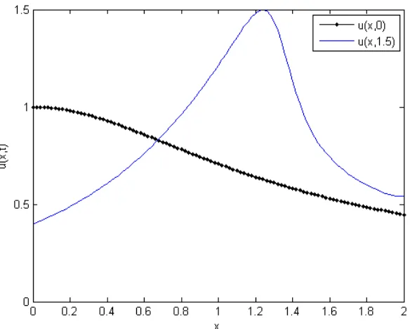
Δ = 0.02. We calculate the numerical solution from the initial time = 0 until the final time = 1.5 with time step _{Δ = 0.5Δ .} For the initial condition we assume ( , 0) = 1/ 1 + . The boundary condition at the left-end is (0, ) = 1/(1 + ), and at the right-end (2, ) is set to be transmissive. The flux function for the Burgers equation here is ( , ) = ( ) ( ) where ( ) = 1/(1 + ) and

( ) = /2 .

Figure 1. Numerical solutions produced using the Lax–Friedrichs finite volume method at = 1.5.

We obtain that the Lax–Friedrichs finite volume method is fast in computation. The Lax–Friedrichs finite volume method only needs 21.4 seconds to compute numerical solutions, even though this running time can still be optimised. Numerical solution of the Lax–Friedrichs finite volume method is shown in Figure 1.

ICSAS IOP Publishing

IOP Conf. Series: Journal of Physics: Conf. Series 795₍₂₀₁₇₎₀₁₂₀₄₃_doi:10.1088/_1742-6596_/₇₉₅_/1/₀₁₂₀₄₃

(6)

4.2. Results of the Jin–Xin relaxation method

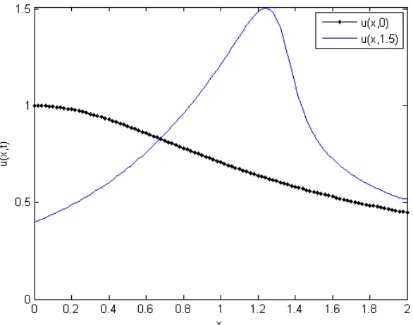
Using the Jin–Xin relaxation method, we compute from the starting point = 0 to final point = 2 with cell width Δ = 0.05. We compute the solution from the initial time = 0 until the final time

= 1.5 with time step _{Δ = 0.01Δ .} The initial and boundary conditions are the same as the previous simulation. The small positive constant (relaxation rate) that we used here is - = 10#3.

Figure 2. Numerical solutions produced using the Jin–Xin relaxation method at = 1.5.

The Jin–Xin relaxation method needs 300.0 seconds to compute numerical solutions. But if we choose _Δ too big, then the method becomes unstable. Numerical results of the Jin–Xin relaxation method are shown in Figure 2 giving similar behaviour to that of the Lax–Friedrichs results.

5. Conclusion

According to our research, the Lax–Friedrichs finite volume method is faster than the Jin–Xin relaxation method in the computation. However, the Jin–Xin relaxation method is easy to compute due to its linear approach. With these results, we suggest that researchers should be aware of these trade-off when they want to take one of these two methods to solve the spatially-varying Burgers equation.

Acknowledgment

This work was financially supported by Sanata Dharma University. The financial support is gratefully acknowledged by both authors.

References

[1] Wiryanto L H and Mungkasi S 2015 Internal monochromatic wave propagating over two bars Applied Mathematical

Sciences 9 4479

[2] Mungkasi S 2016 Adaptive finite volume method for the shallow water equations on triangular grids Advances in

Mathematical Physics 2016 7528625

[3] Wiryanto L H and Mungkasi S 2016 Numerical solution of waves generated by flow over a bump Far East Journal

of Mathematical Sciences 100 1717

[4] LeVeque R J 1992 Numerical Methods for Conservation Laws (Basel: Springer)

[5] LeVeque R J 2002 Finite Volume Methods for Hyperbolic Problems (Cambridge University Press: Cambridge) [6] Mungkasi S, Sambada F A R and Puja I G K 2016 Detecting the smoothness of numerical solutions to the Euler

equations of gas dynamics ARPN Journal of Engineering and Applied Sciences 11 5860

(7)

[7] Supriyadi B and Mungkasi S 2016 Finite volume numerical solvers for non-linear elasticity in heterogeneous media

International Journal for Multiscale Computational Engineering 14 479

[8] Mungkasi S 2015 Some advantages of implementing an adaptive moving mesh for the solution to the Burgers equation IOP Conference Series: Materials Science and Engineering 78 012031

[9] Prnić Ž 1995 Godunov scheme for the scalar nonlinear conservation laws with flux depending on the space variable

Mathematical and Computer Modelling 22 l

[10] Jakawat W, Favre C and Loudcher S 2016 Graphs enriched by cubes for OLAP on bibliographic networks

International Journal of Business Intelligence and Data Mining 11 85

[11] Morano P, Marco Locurcio M, Tajani F and Guarini M R 2015 Fuzzy logic and coherence control in multi-criteria evaluation of urban redevelopment projects International Journal of Business Intelligence and Data Mining 10 73

[12] Tour G and Tangman D Y 2014 Option pricing under a Markov modulated model using a cubic B-spline collocation method International Journal of Business Intelligence and Data Mining 9 356

[13] Jin S and Xin Z 1995 The relaxation schemes for systems of conservation laws in arbitrary space dimensions

Communications on Pure and Applied Mathematics 48 235

[14] Banda M K and Seaid M 2005 Higher-order relaxation schemes for hyperbolic systems conservation laws Journal of

Numerical Mathematics 13 171

[15] Mungkasi S and Christian A 2017 Runge-Kutta and rational block methods for solving initial value problems Journal

of Physics: Conference Series accepted