Behaviour of the numerical entropy production of the one-and-a-half-dimensional shallow water equations.

(1)

ANZIAM J. 54 (CTAC2012) pp.C18–C33, 2013 C18

Behaviour of the numerical entropy production

of the one-and-a-half-dimensional shallow

water equations

Sudi Mungkasi

1

Stephen G. Roberts

2

(Received 18 October 2012; revised 19 March 2013)

Abstract

This article reports the behaviour of the numerical entropy pro-duction of the one-and-a-half-dimensional shallow water equations. The and-a-half-dimensional shallow water equations are the one-dimensional shallow water equations with a passive tracer or transverse velocity. The studied behaviour is with respect to the choice of numer-ical fluxes to evolve the mass, momentum, tracer-mass (transverse mo-mentum), and entropy. When solving the one-and-a-half-dimensional shallow water equations using a finite volume method, we recommend the use of a double sided stencil flux for the mass and momentum, and in addition, a single sided stencil (upwind) flux for the tracer-mass. Having this recommended combination of fluxes, we use a double sided

http://journal.austms.org.au/ojs/index.php/ANZIAMJ/article/view/6243

gives this article, c Austral. Mathematical Soc. 2013. Published May 5, 2013, as part of the Proceedings of the 16th Biennial Computational Techniques and Applications Conference.issn1446-8735. (Print two pages per sheet of paper.) Copies of this article

must not be made otherwise available on the internet; instead link directly to thisurlfor

(2)

Contents C19

stencil entropy flux to compute the numerical entropy production, but this flux generates positive overshoots of the numerical entropy production. Positive overshoots of the numerical entropy production are avoided by use of a modified entropy flux, which satisfies a discrete numerical entropy inequality.

Subject class: 65M08, 65M50, 76M12

Keywords: numerical entropy production, smoothness indicator, re-finement indicator, finite volume methods, shallow water equations, passive tracer, transverse velocity

conservation laws were solved using a finite volume method with the same type of numerical fluxes for the evolutions of all conserved quantities. The numerical flux used by Puppo and Semplice [4] was the Lax–Friedrichs flux, which is a double sided stencil flux. In their work, shallow water equations were not particularly considered.

With a finite volume method to solve the 1.5D swe, we could use the same

type of numerical fluxes having a double sided stencil formulation. However, to get a more accurate solution to the passive tracer or transverse velocity, the strategy is as follows: for the evolutions of conserved quantities of the

1D swewe use the same type of numerical fluxes having double sided stencil

formulations, but for the evolution of the tracer-mass we use the upwind numerical flux (single- sided stencil flux), as suggested by Bouchut [1]. The choice of numerical flux functions to solve the governing equations affects the accuracy of the numerical solutions. Furthermore, the choice of numerical flux functions to solve the governing equations and to evolve the entropy affect the behaviour of the nep.

(4)

2 Governing equations and the numerical entropy production C21

to several combinations of numerical fluxes. With a finite volume method, the numerical fluxes are used to evolve the mass, momentum, tracer-mass (transverse momentum), and entropy for the 1.5D swe.

2

Governing equations and the numerical

entropy production

We present the 1.5Dswe and how we compute thenep. In the 1.5Dswe,

the dynamics of the passive tracer is governed by an additional transport (advection) equation to the 1Dswe. This additional transport equation does

not influence the fluid dynamics of the1Dswe. Note that the concentration of

the passive tracer in the passive tracer framework is in place of the transverse velocity in the transverse velocity framework.

We limit our discussion to shallow water flows on a horizontal topography (without source terms). The1.5D swe are

ht+ (hu)x = 0, (1)

(hu)t+

hu2+1

2gh

2

x

= 0, (2)

(hv)t+ (huv)x = 0. (3)

Here,x represents the coordinate in one-dimensional space, t represents the time variable, g is the acceleration due to gravity, h =h(x,t) denotes the water height, u=u(x,t) denotes the water velocity in the x-direction, and

v(x,t)is the transverse velocity or the concentration of the passive tracer. The transverse velocity is orthogonal to the x-axis and has a horizontal direction. The conserved quantities of the 1.5D swe are the mass or water height h,

(5)

2 Governing equations and the numerical entropy production C22

The entropy inequality for (1)–(3) is

ηt+ψx 60, (4)

where the entropy (the physical energy) η and the entropy flux (the flux of the physical energy)ψ are

η(q(x,t)) = 1

2h(u

2₊_v2_{) +} 1

2gh

2_, ₍₅₎

ψ(q(x,t)) =

1 2h(u

2₊_v2_{) +}_gh2

u, (6)

andq(x,t) = (h hu hv)T _{is the vector of conserved quantities of the}₁_.₅_D_swe_.

Inequality (4) is to be understood in the weak sense. For smooth solutions, inequality (4) becomes an equation and is called the entropy equation. For nonsmooth solutions, it becomes a strict inequality. Inequality (4) is described in further detail by Bouchut [1], amongst others.

We adapt the existing numerical entropy scheme described in our previous work [3]. The numerical entropy production (nep) in the jth cell at the

nth time step is

En_j = 1

∆t

η Qn_j−Θn_j

, (7)

which is the local truncation error of the entropy at the corresponding cell and the corresponding time. Here, Θn

j is an approximation of the average

of the exact entropy η in the jth cell at the nth time step and calculated using the numerical entropy scheme with η Qn−1

as the input, Qn_j is an approximation of the average of the exact quantityqj(x,tn) in the jth cell

at the nth time step (t =tn_{) and calculated using the numerical conserved}

quantity scheme withQn−1 _{as the input, and}_∆t_{is the time step used in both}

(6)

3

Flux functions for finite volume methods

This section provides three combinations of numerical flux functions for finite volume methods used to solve the 1.5D swe.

Conservation laws

qt+f(q)x =0 (8)

are solved using a first order finite volume method [2]

Qn+1 j =Q

n j −λ

Fn_j₊1 2

−Fn_j₋1 2

. (9)

HereF_j+1₂ andFj−1₂ are numerical fluxes of the conserved quantities computed in such a way that the method is stable with λ = ∆t/∆x. Variables ∆t

and∆xare the time step and cell-width. We assume that the spatial domain is discretised uniformly into a finite number of cells. The notationQn

j represents

an approximation of the average of the exact quantityqj(x,tn)in thejth cell

at the nth time step. In addition, fis the analytical flux function.

For our numerical experiments on the 1.5D swe, we consider a double sided

stencil flux function and a single sided stencil flux function. In particular, we take the local Lax–Friedrichs flux and the upwind flux functions for numerical evolutions. As a double sided stencil flux, the local Lax–Friedrichs flux function is suitable for the evolution of all quantities (mass, momentum, tracer-mass, and entropy). As a single sided stencil flux, the upwind flux function is suitable for the evolution of the tracer-mass.

We consider three combinations of flux functions in our numerical schemes, namely:

A local Lax–Friedrichs flux for the mass, momentum, tracer-mass, and

entropy evolutions;

B local Lax–Friedrichs flux for the mass, momentum, and entropy

(7)

C local Lax–Friedrichs flux for the mass and momentum evolutions,upwind

flux for the tracer-mass evolution,modified flux for the entropy evolution.

For our reference, we call these combinations of flux functionsCombination A,

Combination B, and Combination C, respectively.

In the evolution of the numerical conserved quantity scheme and the numerical entropy scheme, we can simply use the same type of flux function (in particular the local Lax–Friedrichs flux as we mentioned above) for evolving the mass, momentum, tracer-mass, and entropy. This motivates Combination A.

The local Lax–Friedrichs fluxes used for Combination A are described as follows. Consider thejth cell, which is the interval(x_j−12,xj+

1

2)of the uniformly discretised spatial domain. The local Lax–Friedrichs flux for the quantity evolution has the form [2,4]

Fn_j₊1

2 =F(Q

n j+1,Q

n j) =

1 2

h

f Qn_j+1

+f Qn_j

−αn_j₊1 2 Q

n j+1−Q

n j

i

(10)

where αn j+12

= max|un j+1|+

p

ghn j+1, |u

n j|+

p

ghn j

is the coefficient of ar-tificial diffusion, chosen at each time step locally. Notations un

j and hnj

represent the numerical velocity and water height, respectively, in the jth cell at the nth time step. Recall that Qn

j is an approximation of the average

of the exact quantity qj(x,tn) in the jth cell at the nth time step. The

notation q, or qj for the specific jth cell, represents the mass, momentum,

or tracer-mass. Furthermore, the local Lax–Friedrichs flux for the entropy evolution is

Ψn_j₊1

2 =Ψ(Q

n j+1,Q

n j) =

1 2

ψ Qn_j+1

+ψ Qn_j−αn_j₊1 2

η Qn_j+1

−η Qn_j

(11) where Qn_j is an approximation of the average of the exact conserved quan-tityqj(x,tn)in the jth cell at thenth time step. To make the notation clear,

we note that Qn_j = [hn_j (hu)n j (hv)

n j]

T_{, where} _hn

j is an approximation of the

average of water height h in the jth cell at the nth time step. The notations (hu)n

(8)

To get a more accurate solution of the tracer, a natural way is by using the upwind flux function for the evolution of the tracer-mass [1]. This leads to CombinationB: the local Lax– Friedrichs flux for the mass, momentum, and entropy; and the upwind flux for the tracer-mass. For Combination B, the local Lax–Friedrichs flux for the mass and momentum is defined by (10). The local Lax–Friedrichs flux for the entropy is defined by (11). The upwind fluxFn,hv

j+1₂ for the tracer-mass at the spatial point x=xj+ 1

2 at timet =t

n _is

Fn,hv

j+12 =

 



Fn,h

j+1₂vj if F

n,h

j+1₂ >0,

Fn,h

j+1₂vj+1 otherwise .

(12)

Here Fn,h

j+1₂ is the mass flux computed using the local Lax–Friedrichs flux (10) at the spatial point x=x_j+1₂ at timet =t

n_.

In our numerical results presented in the next section (Section4), we see that Combination B leads to positive overshoots of the nep. To avoid positive

overshoots of the nep, the entropy flux is modified with respect to the local

Lax–Friedrichs and upwind flux functions, because these two fluxes are used in the numerical conserved quantity scheme. With a particular modification of the entropy flux, the entropy evolutions satisfy a discrete numerical entropy inequality as described by Bouchut [1]. This leads to Combination C: the local Lax–Friedrichs flux for the mass and momentum, the upwind flux for the tracer-mass, and the modified flux for the entropy. For CombinationC, the local Lax–Friedrichs flux for the mass and momentum is defined by (10). The upwind flux for the tracer-mass is defined by (12). The modified flux for the entropy is

Ψn_j₊1 2

=Ψn,1d

j+1₂ +Ψ

n,hv

j+1₂ . (13)

Here, Ψn,1d

j+1₂ is a numerical entropy flux of the1Dswe part at thenth time step. In our case Ψn,1d

j+1₂ is computed using the Lax–Friedrichs entropy flux, that is, the numerical entropy flux of the form (11) with setting v=0. In addition, Ψn,hv

(9)

Ψn,hv

j+1₂ is computed using the upwind entropy flux

Ψn,hv

j+1₂ = ₁

2F n,h

j+1₂v

2

j if F n,h

j+1₂ >0,

1 2F

n,h

j+1₂v

2

j+1 otherwise .

(14)

This modified numerical entropy flux is adapted from Bouchut [1, equation (3.88) for more detail].

4

Numerical experiments

This section presents numerical results relating to the behaviour of the nep

of the 1.5D swe. The three combinations, A, B and C, of flux functions are

tested.

For our experiments, the numerical setting is as follows. First order methods are implemented. All variables are quantified in si units. The acceleration

due to gravity is taken as g=9.81. The Courant–Friedrichs–Lewy number is1.0. The discrete L1 _{relative error}

ELQ1 = PN

j=1

q(x_j,tn) −Qn_j

PN

j=1|q(xj,tn)|

(15)

is used to quantify numerical errors, whereNis the number of cells,q(xj,tn)is

the exact quantity at (x,t) = (xj,tn), and Qnj is an approximation of the

average of the exact quantity qj(x,tn) in the jth cell at the nth time step.

The term “quantity” in this case represents the water mass (height) h, momentum hu, transverse momentum (tracer-mass) hv, velocity u, and transverse velocity (the concentration of the passive tracer)v. Note that the notation q(xj,tn) is different from qj(x,tn).

(10)

considered. The initial condition is

u(x,0) = 0, (16)

v(x,0) =

3 if −2000 < x < 0,

0 if 0 < x < 2000, (17)

h(x,0) =

10 if −2000 < x < 0,

4 if 0 < x < 2000. (18)

This initial water height h(x,0)is chosen in such a way that we clearly see a rarefaction, a contact discontinuity (a discontinuity between two different concentrations of the passive tracer), and a shock wave propagate at time

t > 0. We could take a much smaller initial water height for 0 < x < 2000, but the contact discontinuity and the shock wave would not be clearly seen, because the rarefaction would dominate the water motion at time t > 0. The exact analytical solution of the dam break problem was derived by Stoker [5]. LeVeque [2] reviewed shallow flows with a passive tracer. .

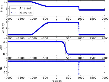
A comparison of numerical errors is given in Table1. From Table1, Combina-tions A,BandC lead to exactly the same results (and hence the same errors) in h and u. Combinations B and C lead to exactly the same results in v, while Combination Aleads to larger errors of v than the errors of vproduced by CombinationsB and C. As the cells are uniformly refined, the errors get smaller and the numerical solutions better approximate the exact solution. Even though we use first order methods, the convergence is not of order of one, but less than one. This convergence is due to discontinuities occurring in the numerical solutions. We summarise in Table 1, Combinations B andC generate more accurate results and they have the same performance.

(11)

5 Conclusions C28

Table 1: Errors of h, u and v resulting from a finite volume method with

fluxes using Combinations A, B and C for various numbers of cells. The

errors are quantified att =100.

number h error uerror v error v error of cells A, B, C A, B, C A B, C

100 0.019 0.108 0.070 0.037 200 0.012 0.066 0.050 0.026 400 0.007 0.038 0.035 0.019 800 0.004 0.022 0.025 0.013 1600 0.002 0.013 0.018 0.009

nepin Figure 1. We restate that Combinations A and B lead to the same

results in h and u, but Combination B gives more accurate results in v(see Table 1). However, Combination B produces positive overshoots and an oscillation of thenep around the contact discontinuity, as shown in Figure 2.

Furthermore, Combinations B and C produce the same errors inh, uand v, but no positive overshoots of the nep are generated by Combination C as

shown in Figure 3. In addition, Figure 2suggests that Combination B results in a solution which does not satisfy a discrete entropy inequality, whereas Figures 1and3 suggest that Combinations AandC result in solutions which satisfy a discrete entropy inequality.

5

Conclusions

(12)

5 Conclusions C29

−2000 −1500 −1000 −500

0

500

1000 1500 2000

5

10

Sta

ge

Ana sol

Num sol

−2000 −1500 −1000 −500

0

500

1000 1500 2000

2

4

Ve

loc

ity

−2000 −1500 −1000 −500

0

500

1000 1500 2000

0.0

1.5

3.0

v(x

)

−2000 −1500 −1000 −500

0

500

1000 1500 2000

Position

-20

-10

0

NE

P

Figure 1: Results of a simulation using Combination A with 1600 cells at

time t=100. The nep (7) is nonpositive everywhere. “Ana sol” and “Num

sol” stand for analytical solution and numerical solution, respectively.

(13)

5 Conclusions C30

−2000 −1500 −1000 −500 0 500 1000 1500 2000 Position

-20 -10 0

N

EP

Figure 2: The nep (7) resulting from Combination B with 1600 cells at

t =100. Positive overshoots of the nep are generated around the contact

discontinuity.

around a contact discontinuity. If we use a flux modified in such a way that a discrete numerical entropy inequality is satisfied, then no positive overshoots of the numerical entropy production are produced.

(14)

5 Conclusions C31

−2000 −1500 −1000 −500 0 500 1000 1500 2000 Position

-20 -10 0

N

EP

Figure 3: The nep (7) resulting from Combination C with 1600 cells at

t=100. Thenep is nonpositive everywhere.

is implemented in an adaptive-mesh finite volume method as the refinement (smoothness) indicator, these positive overshoots and the oscillation of

(15)

References C32

Acknowledgements The work of Sudi Mungkasi was financially supported by The Australian National University. We thank Professor Sebastian Noelle of

Institut f¨ur Geometrie und Praktische Mathematik, RWTH Aachen University,

Germany for some discussions, and Professor Randall John LeVeque of the Department of Applied Mathematics, the University of Washington, USA for some comments.

References

[1] F. Bouchut. Efficient numerical finite volume schemes for shallow water models. In V. Zeitlin (editor), Nonlinear dynamics of rotating shallow

water: methods and advances, Volume 2 of Edited series on advances in

nonlinear science and complexity, pages 189–256. Elsevier, Amsterdam, 2007. http://dx.doi.org/10.1016/S1574-6909(06)02004-1 C20, C22, C25, C26

[2] R. J. LeVeque. Finite-volume methods for hyperbolic problems. Cambridge University Press, Cambridge, 2002.

http://dx.doi.org/10.1017/CBO9780511791253 C20, C23, C24,C27

[3] S. Mungkasi and S. G. Roberts. Numerical entropy production for shallow water flows. ANZIAM Journal, 52(CTAC2010):C1–C17, 2011.

http://journal.austms.org.au/ojs/index.php/ANZIAMJ/article/ view/3786/1410 C22

[4] G. Puppo and M. Semplice. Numerical entropy and adaptivity for finite volume schemes. Communications in Computational Physics,

10(5):1132–1160, 2011.

http://dx.doi.org/10.4208/cicp.250909.210111a C20, C24, C30

(16)

References C33

http://onlinelibrary.wiley.com/book/10.1002/9781118033159

C27

Author addresses

1. Sudi Mungkasi, Mathematical Sciences Institute, The Australian National University, Canberra, Australia; Department of Mathematics, Sanata Dharma University, Yogyakarta, Indonesia.

mailto:sudi.mungkasi@anu.edu.au;sudi@usd.ac.id

2. Stephen G. Roberts, Mathematical Sciences Institute, The Australian National University, Canberra, Australia.