405
International Journal of Mechanical and Materials Engineering (IJMME), Vol.6 (2011), No.3, 405-413
STRESS WAVE METHOD FOR IDENTIFICATION OF VISCOELASTIC MATERIAL
PROPERTY BASED ON FINITE-ELEMENT INVERSE-ANALYSIS
F.E. Gunawan
Jl KH Syahdan 9, Jakarta 11480, Indonesia
Industrial Engineering Department, Faculty of Engineering, Bina Nusantara University Email: [email protected], [email protected]
Received 28 September 2011, Accepted 15 December 2011
ABSTRACT
This paper proposes a procedure to identify the viscoelastic material constants using the inverse analysis and the finite element analysis. The procedure requires two measured data: the applied impact-force and the structural elastic response at a point, and further assumes the material viscoelasticity following the Prony series expansion. In this procedure, we infer the viscoelastic material constants in the following steps: we initialize the viscoelastic material constants, and then calculate the stress state at the point, and finally, we check the equilibrium of the constitute equation. The procedure is repeated until the equilibrium of the constitute equation is satisfied. In this repetition, the viscoelastic material constants are updated following the Gauss-Newton method. In addition, we evaluated the method by using data obtained from a simulated impact on a viscoelastic plate, and the results were rather promising. Finally, we studied the convergence of the procedure using various random material constants as the input data.
Keywords: Visco-elasticity, Stress-wave, Inverse-problem, Finite element method
1. INTRODUCTION
The viscoelastic materials are playing an important role in many engineering structures. Those materials such as polymers (Drozdiv and Dorfmann, 2002) are being used, for examples, to dissipate and to insulate vibration caused by rotating or reciprocal movement. It also has potential application in a new Hopkinson pressure bar testing apparatus (Zhao and Gary, 1995; Zhao et al., 1997; Salisbury, 2001; Benatar et al., 2003; Casem et al., 2003). Therefore having the data of the material, particularly related with their mechanical characteristics, are essential. Unfortunately, identifying those data are often not easy due to limitation enforced by the standard testing procedure. American Society for Testing and Materials devised ASTM E139-06 Standard Test Methods for Conducting Creep, Creep-Rupture, and Stress-Rupture Tests of Metallic Materials is, unfortunately, only suitable for an extremely low loading rate. Another standard test, ASTM D6048-07 Standard Practice for Stress Relaxation Testing of Raw Rubber, Unvulcanized Rubber Compounds, and Thermoplastic Elastomer, is only suitable for a certain
specimen design and well-specified loading technique. Neither standard can be used on medium to high strain rate loading condition, or on a thin film polymer specimen (Ju and Liu, 2002).
406
two, one should rely on a wave propagation method (Blanc, 1993). Many existing wave propagation methods exploit the benefit of the simplicity of the wave propagation theory in one dimension (see, for examples, Kolsky (1963); Graff (1975); Doyle (1989)). This phenomenon can be observed in a slender bar specimen subjected to a pulse impact-force. Using the bar specimen, Blanck (Blanc, 1993), Lemerle (Lemerle, 2002), and Lundber and Blanc (Lundberg and Blanc, 1988) demonstrated that viscoelastic property could be inferred from some mechanical responses such displacement or strain at two different locations. The inference is on the basis of the following formula:
)
is the phase angle of the quantity (the displacement of the strain), is the angular frequency, and c() is the phase
velocity. And then, the wave speed is used to compute the complex Young's modulus. Hilton et al. (2004) argued that the viscoelastic material constants could be identified by inversely solving the convolution integral for viscoelastic material derived by Christensen (1981) using the elastic-viscoelastic analogy. However, until this time, it is still very difficult to convert the complex Young's into the Young's modulus in the time domain. Expressing the property in the time domain is necessary because the existing mechanics for viscoelastic materials is much well-established in the time domain than that in the frequency domain (see, for examples, (Zienkiewics and Taylor, 2000, Section 3.2 Viscoelasticity) and (Mesquite and Code, 2003)). Furthermor existing commercial finite element packages such as ANSYS (Kohnke, 1999) and ABAQUS (Abaqu2008) require a user to supply the material data in the time domain. Those reasons are major limitation of the existing identification method in the group of the wave propagation. In addition, the method is only applicable when the involved wave length is much longer than the largest dimension of the specimen cross section. Soderstrom (2002) shows that if the wave length is longer than 10d, where
d is the specimen diameter, then the valid frequency range is smaller than c/(10d), where c is the longitudinal wave speed. However, this limitation is due to the underlying theory where Eq. (1) was derived, and it seems to us, this limitation can be avoided when a higher order approximation, see for an example Anderson (2006), is used in deriving the governing dynamics.
This work aims to develop a new technique to identify the viscoelastic material property within the wave propagation method. It is designed to overcome limitations mentioned above. In addition, the technique allows one to use a more complex specimen geometry such as a plate specimen; On some circumstances, such a specimen geometry is more preferable. Therefore, the method does not limit the valid
frequency range of the stress-wave involved during the test. We should note that the underlying theory used in deriving the equation of motion often strictly limits the use of the theory such as those in the slender bar case.
In the present work, we combine the finite element method and the nonlinear least-squares method to infer the viscoelastic material property. In general, the use of such approach is not completely new; Aoki et al. (1997), for an example, has adopted the approach to infer the Gurson material constants because those data are difficult to be measured directly from an experiment. In addition, Mahata et al. (2004); Mahata and Soderstrom (2004) employed the nonlinear least-squares method to establish a non-parametric wave propagation function in the frequency domain. Matzenmiller and Gerlach (2001) utilized the correspondence principle of viscoelastic materials and a numerical technique to inverse the relaxation function in the Laplace domain. They also assumed that the material bulk modulus does not depend on time; the same assumption is used in this work. A more common approach is to parametrize the material property function such as using a Prony series (Tschoegl, 1989), and the parameters are determined accordingly. Emri and Tschoegl (1993) presented a recursive computer algorithm technique to determine the relaxation time from relaxation modulus data. Subsequently, Tschoegl and Emri (1993) also utilized the theoretical storage and loss functions, and demonstrated using experimental data (Emri and Tschoegl, 1994, 1995).
2. MECHANICAL BEHAVIOR OF VISCOELASTIC MATERIALS
2.1 General
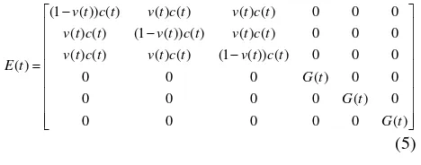
The state of stress in an elemental volume of a loaded body is defined in terms of six components of stress, and expressed in a vector form as
TCorresponding to the six stress components in Eq. (2) is the state of strain, which can also be written in a vector:
TUsing the elastic-viscoelastic analogy Christensen (1981), the theory of elasticity has been extended to the viscoelastic material. For the viscoelastic material, the material properties are a function of time and the past response affecting the present stress state. Both the phenomena can be expressed by a hereditary integral:
407
For general viscoelastic material in small deformation regime, the dilatational modulus and the shear modulus should be assumed to be a function of time. However, there are many engineering material where the dilatational deformation does not depend on time (Flugge, 1975). Hence, the dilatation deformation is completely elastic
Ke be sought. The viscoelastic stress-strain relationship can also be written in form of compliance function:
, which are generaly applicable.
2.2 Parameterization by Prony Series Expansion
When the data of the stress (Eq. (2)) and the strain (Eq. (3)) at a point exist, Eq. (4) or Eq. (9) can be used to obtain the material data E(t) or G(t). However, solving the both
equations inversely are not easy due to the numerical stability. Such as a process is called deconvolution, and its results are often sensitive to the data error depending on the condition number of the problem. Parameterization of the unknown variable in a deconvolution often leads to much accurate solution as demonstrated in Gunawan et al. (2006). Fortunately, parameterization of the viscoelastic material, such as using Prony series expansion, has been widely used in representing the viscoelastic characteristics. The Prony
series expansion of the shear relaxation G(t) is given by a
series of the exponential function:
solid viscoelastic material is obtained. The model has three unknown parameters, and it is capable to express the stress relaxation or the strain retardation phenomena of many solid viscoelastic materials particularly within a short range of time. For the standard linear solid model, the shear relaxation function can be reduced to discussion, following Emri and Tschoegl (1997)'s advise, that for the time duration of interest of 100 s , only one Maxwell unit is relevant, and the related constants need to be determined.
3. INVERSE ANALYSIS FOR MATERIAL
PROPERTY IDENTIFICATION
To simplify derivation of the present approach, we utilize a simple experimental setup as shown in Fig. 1; however, the technique is also applicable for more complex specimen geometry as demonstrated in Section 4.
Figure 1 A uniaxial impacted bar.
408
G , and so that the differences between G(t) obtained by
Eq. (4) and by Eq. (11) are minimum. It is clear that the necessary data for the calculation are the stress and the strain at the same location. Although, the strain can be easily measured by a strain-gage, but the stress is not easily evaluated, especially for a rather complex structure.
To circumvent such difficulty, the finite element analysis is employed. The experimental setup shown in Fig. 1 is quite simple and the applied load P(t) and (t) can be measured
in the experiment. The stress at the measurement point can be computed by a finite element method for the presumed viscoelastic material constants as the first approximation. The measured strain (t) is taken as the reference strain
) (t
r
; therefore, an error vector can be established as:
' '
) ' ( ) ' ( ) ( ) ( ~
0
dt t
t t t E t
t r
t
r
(13)
In the subsequent iterations, we minimize the error function, in the least-squares sense, by adjusting the material constants using Gauss-Newton method and adjusting the stress using the finite element method. The process is repeated until
2
) ( ~ t
r
is smaller than a certain limit . The detail of the technique is presented chronologicaly in Algorithm 1.
A few notes needs to be outlined regarding Algorithm 1. The data involved in a high impact test often are quite large in size. Therefore, the convolution equation of Eq. (13) must be solved as quickly as possible. By applying the convolution theorem, the equation can quickly be solved in the frequency domain. And, the data can be transformed into the frequency domain using the fast Fourier transformation (Brigham, 1974). However, prior the transformation, zeros as long as the data length should be padded to the tail of data r and to improve the accuracy of the data spectrum in the frequency domain. In addition, because the magnitude of strain is significantly smaller than the stress, those data have to be normalized prior the optimization process, otherwise the Gauss-Newton algorithm may fail to converge. And as a final note, in the present implementation, the central difference approach is used to compute the time derivative of the stress.
A similar procedure can also be used to minimize the error function on the basis of the compliance function of Eq. (14); the both will be evaluated numerically in this work.
) ( ' '
) ' ( ) ' ( ) ( ~
0
t dt t
t t t C
t r
t
r
(14)
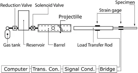
3.1 Experimental Apparatus and Procedures
The experimental apparatus depicted in Fig. 2 is one of many possible arrangements to perform the experiment for
this purpose. In this arrangement, a short-stress pulse is generated by striking the load transfer rod with a ball. The generated stress pulse can be measured using a pair of gages attached to the load transfer road. The gages should be connected to the Wheatstone bridge in a half-bridge configuration; hence, the strains due to the bending wave, if any, could be canceled out.
The data from the bridge will be recorded in a computer via a transient converted and a signal conditioner. The transient converter allows us to temporarily store the data; it becomes necessary particularly when the data need to be sampled at an extremely high rate. Modern signal conditioner usually has filter feature, which is usefull if the data containing excessive noise.
409
4. NUMERICAL EVALUATIONSWe have verified the above procedure using a number of specimen types such as a bar specimen, a one-point bend specimen, and a plate specimen. However, only the results for the case of the plate specimen are presented due to limitation of the space. This particular case is also used to illustrate the proposed procedure.
4.1 Data for Validation
In this section, we present the forward analysis to establish data for verification the proposed procedure and to select the objective function among the existing options of Eq. (13) and Eq. (14). The analysis was performed numerically using the finite element method so that the necessary data could be obtained in a well-controlled environment. However, further verifications on the basis of experimental data are certainly necessary.
The specimen geometric data, material properties, and loading conditions are following: the specimen shape is a square plate with the edge length of 500 mm, and a thickness of 10 mm. The specimen is assumed to be hanged in the air, and is made of a viscoelastic material with following properties: G0 = 161.54 GPa, G= 16.154 GPa, and = 20s, and K= 175.0 GPa. A concentrated load is applied to the middle of the specimen edge where the load varies with time following a half-sine function with a loading duration of 50s. A strain gage is assumed to be attached at a point located 50 mm ahead of the impact-site. This experimental design leads to specimen response where the incident stress-wave can clearly be separated from the reflected stress-wave. This issue is crucial because when the reflected wave superimposing the incident stress-wave, the structural response become too complex, and convergence is hard to be attained.
The above impact event is performed numerically using finite element analysis where the finite element mesh of the model is shown in Fig. 3. Only a half of the specimen is modeled due to symmetry. The model mesh has 5000 linear solid elements and 5151 nodes. Although the event is performed numerically, but it is certainly easy to establish an experimental apparatus for such a case where a short stress-pulse can be produced using a small sphere projectile and the plate specimen can be hanged on the air. The finite element analysis is conducted for various time-steps and various element sizes, and their effects on the stress and the strain at selected measurement point in the analyzed structure are studied. The largest time-step and element-size that do not substantially affect the computed stress and strain are selected for the next analysis. This selection of the time-step and element-size must be carefully made to save the computation time, because the present approach requires that the finite element analysis have to be performed for a few times. From the analysis, we obtain the stress (see Fig. 5) and the strain (see Fig. 4) as a function of time at the
measurement location. In addition, to accommodate the error that inherently exists in the measurement process, small pseudo-random noises are superimposed to the data.
Figure 3 Finite element mesh of a square plate.
Figure 4 The strain time history in x-direction obtained by the finite element analysis (solid line) and those by solving
Eq. (9) (dotted line).
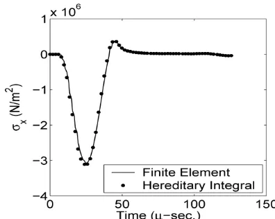
Figure 5 The stress time history in x-direction obtained by the finite element analysis (solid line) and those by
410
It is important to select the best objective function between Eqs. (13) or (14). For a given strain shown in Fig. 4, the hereditary integral of Eq. (4) is solved to obtain the stress presented in Fig. 5 with the dotted line. In the similar manner, the dotted line in Fig. 4 is obtained by solving Eq. (9). Figures 4 and 5 show that the strain computed (dotted line in Fig. 4) from the stress data (solid line in Fig. 5) is less accurate than the stress computed (dotted line in Fig. 5) from the strain data (solid line in Fig. 4). The phenomenon seems to be clear by considering the fact that the displacement-based finite element analysis produces the more accurate strain than the stress. Because of this fact, Eq. (13) is selected as the objective function.
4.2 Inverse Analysis for Identification of Material Constants
In the inverse analysis, the required data are the reference strain
r(t), which are depicted in Fig. 4 with a solid line. To create realistic `measured data', a small amount of the normally distributed pseudo-random noise is superimposed to the data. The ratio of noise to the data is taken as 1.0%. Another required data are initial assumptions of the viscoelastic material constants. Because this data will be used in the finite element analysis, the initial data should reasonably represent the exact viscoelastic constants of a given material. Too small initial data of G0 and G could lead to an un-compressible material and ``hour glassing'' may occur during deformation, while too large initial data may cause the ``locking''. One best way is to employ the data obtained from a static test for the initialization. Theoretically, long-term response of a viscoelastic solid will approach to its elastic response. Therefore, the G can beinitialized with the static shear modulus, in the present case
8 . 80
G GPa. The G0 must be larger than G, so then we assumed G088.0 GPa, or 10.0% higher than the final
shear modulus. The initial relaxation time is taken as 1.0s, which is the same as the sampling-time in the finite element analysis. The time is also a logical choice by considering the duration of the impact-force. It is certainly impossible to identify the relaxation time longer than the loading duration even of the data actually exists. Therefore, the initial design variable is x0
88.0 80.0 1.0
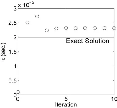
. The strain data presentedin Fig. 4 are utilized, and Algorithm 1 is evaluated for 10 iterations. Figures 6 to 8 show the evolution of the estimated viscoelastic constants along the iterations. On each iteration, the finite element analysis is performed to update the stress, and several sub-iterations are performed to update the viscoelastic material constants. In Fig. 9, the estimated shear modulus at the 10-th iteration is compared to the exact shear modulus. Although the shear relaxation function shows a relatively good agreement, the estimated viscoelastic material constants converge to a certain value slightly deviated from the exact data.
Figure 6 Estimated instantaneous shear modulus along iteration
Figure 7 Estimated final shear modulus along iteration
411
Figure 9 Comparison of estimated and exact shear relaxation function
4.2.1 Convergence of the Finite-Element Inverse-Analysis
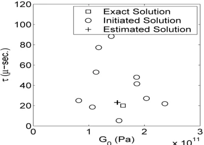
Numerical results in Figs. 6 to 8 indicate that the combined finite-element inverse-analysis method has a fast rate of convergence. Following, we study the robustness of the method particularly with respect to the initial data. The robustness is examined with respect to the ability of the procedure to consistently converge for given any initial data in the feasible domain. For this purpose, wide ranges of initial data of the viscoelastic material constants are provided. The initial data of the initial shear modulus is selected from normally distributed pseudo-random numbers in the range of the elastic shear modulus to five times larger than the elastic shear modulus. The initial data of the final shear modulus is set as the same with the exact final shear modulus. The initial relaxation time is randomly selected from uniformly distributed random numbers in the range of the sampling time to the whole analysis time. For each set of initial data, the analysis of Algorithm 1 is performed for 5 iterations. Ten data sets are used for the evaluation. The results are presented in Fig. 10, and it is seen that the convergence of the Algorithm 1 is consistent and falls within a reasonable degree of accuracy.
Figure 10 Convergence map of G0 and
4.2.2 Effect of the Loading Rate
The coupling method of finite element and inverse analysis can identify the viscoelastic material constants using the data of viscoelastic response of the structure. If the structure is statically loaded, the response data will not contain the viscoelastic property, i.e., the stress relaxation and the strain retardation. Consequently, such data cannot be used to identify the viscoelastic material constants. This fact suggests that the loading rate affects the accuracy in the estimation of viscoelastic material constants. Different loading rate can be obtained by varying the loading duration. The shorter loading duration provides the higher loading rate. In this section, the effect of loading duration,load, on accuracy of the estimated viscoelastic material constants is examined. The loading profile is assumed to be similar to the profile of a half-sine function. The loading duration is varied to 40, 50, 75 and 100 s , and for each case, the analysis is performed for 100 s . It is easy to produce such variation of the loading duration, for an example, by changing the length of the impact.The results, summarized in Table 1, suggest that the estimated initial shear modulus, final shear modulus and the relaxation time are slightly affected by the loading duration.
Table 1 Effect of the loading duration to the estimated viscoelastic material constants
s) (
load
Exact0 0/G
G G/GExact
/
Exact0 0.94 0.93 1.15 50 0.93 0.93 1.13 75 0.92 0.93 1.12 100 0.91 0.90 1.11
5 CONCLUSIONS
A new method is proposed to identify the parameters of a simple viscoelastic model in form of the Prony series expansion. The method is basically based on a coupling of the finite element analysis and inverse analysis. The method estimates the parameters by minimizing discrepancy of the stress-time histories—utilizing the Gauss-Newton method— at a reference point selected by the user. It takes advantages of the finite element analysis; hence, the proposal, unlike the existing methods, is also suitable for complex specimen geometry. However, verification on the basis of experimental data for various specimen geometries is necessary to further assess the accuracy and robustness of the proposal.
REFERENCES
Abaqus (2008). ABAQUS Analysis User's Manual Version 6.8.
412
elastic bars, Journal sound and vibration, 290: 290— 308.
Aoki, S., Amaya, K., Sahashi, M., and Nakamura, T. (1997). Identification of gurson's material constants by using Kalman filter. Computational Mechanics, 19(6): 501—506
Araujo, A. L.; Soares, C. M. M.; Soares, C. A. M. & Herskovits, J. (2010). Characterisation by inverse techniques of elastic, viscoelastic and piezoelectric properties of anisotropic sandwich adaptive structure, Applied composite materials, 17: 543—556.
Barkanov, E.; Skukis, E. and Petitjean, B. (2009). Characterisation of viscoelastic layers in sandwich panels via an inverse technique, Journal of sound and vibration, 327: 402—412.
Baumgaertel, M., and Winter, H., (1989). Determination of discrete relaxation and retardation time spectra from dynamics mechanical data. Rheological acta, 28: 511—519.
Benatar, A., Rittel, D., and Yarin, A. (2003). Theoretical and experimental analysis of longitudinal wave propagation in cylindrical viscoelastic rods. J. of the mechanics and physics of solids, 51: 1413—1431. Blanc, R.H. (1993). Transient wave propagation methods
for determining the viscoelastic properties of solids. Journal of applied mechanics, 60: 763—768.
Brigham, E.O. (1974). The Fast Fourier Transform. Prentice-Hall, Inc., Englewood Cliffs, New Jersey. Casem, D.T., Fourney, W., and Chang, P. (2003). Wave
separation in viscoelastic pressure bars using single-point measurements of strain and velocity. Polymer testing, 22: 155—164.
Casimir, J.B. and Vinh, T., (2012). Measuring the complex moduli of materials by using the double pendulum system, Journal of sound and vibration, 331: 1342— 1354.
Christensen, R.M. (1981). Theory of viscoelasticity. Academic Press, New York, 2nd edition.
Doyle, J.F. (1989). Wave Propagation in Structures: an FFT-based spectral analysis methodology. Springer-Verlag, New York.
Drozdiv, A.D. and Dorfmann, A. (2002). The nonlinear viscoelastic response of carbon black-filled natural rubbers. International journal of solids and structures, 39: 5699—5717.
Emri, I., and Tschoegl, N.W. (1993). Generating line spectra from experimental responses. part I: relaxation modulus and creep compliance. Rheologica Acta, 32: 311—321.
Emri, I., and Tschoegl, N.W. (1994). Generating line spectra from experimental responses. part IV: application to experimental data. Rheological Acta, 33:60—70.
Emri, I., and Tschoegl, N.W. (1995). Determination of mechanical spectra from experimental responses. International Journals of Solids and Structures, 32:817—826.
Emri, I., and Tschoegl, N.W. (1997). Generating line spectra from experimental responses. part V: Time-dependent viscocity. Rheologica Acta, 36:303—306. Flugge, W. (1975). Viscoelasticity. Springer-Verlag,
second revised edition.
Graff, K.F. (1975). Wave Motion in Elastic Solids. Ohio State University Press.
Gunawan, F. E., Homma, H., and Kanto, Y. (2006). Two-step b-splines regularization method for solving an ill-posed problem of impact-force reconstruction. Journal of Sound Vibration, 297:200—214. doi: 10.1016/j.jsv.2006.03.036.
Hillstrom, L., Mossberg, M., and Lundberg, B. (2000). Identification of complex modulus from measured strains on an axially impacted bar using least squares. Journal of sound and vibration, 230(3):689—707. Hilton, H. H., Beldica, C.E., and Greffe, C. (2004). The
relation of experimentally generated wave shapes to viscoelastic material characterizations—analytical and computational simulations. http://www.ncsa.uiuc.edu/ Divisions/Communities/ CSM/ publications/ 2001/ASC.01.pdf (Retrieved on December 15, 2004). Ju, B.F., and Liu, K.K. (2002). Characterizing viscoelastic
properties of thin elastometic membrane. Mechanics of materials, 34:485—491.
Kim, Sun-Yong and Lee, Doo-Ho (2009). Identification of fractional-derivative-model parameters of viscoelastic materials from measured FRFs, Journal of sound and vibration, 324:570—586
Kohnke, P. (1999). ANSYS Theory Reference. ANSYS, Inc., eleventh edition; release 5.6 edition. Chapter 4.6. Kolsky, H. (1963). Stress Waves in Solids. Dover
Publication, Inc., New York.
Lemerle, P. (2002). Measurements of the viscoelastic properties of damping materials: adaptation of the wave propagation method to test samples of short length. Journal of sound and vibration, 250(2):181— 196.
Lundberg, B., and Blanc, R.H. (1988). Determination of mechanical properties from two-point response of an impact linearly viscoelastic rod specimen. Journal of sound and vibration, 126(1):97—108.
Mahata, K., and T. Soderstrom, T. (2004). Improved estimation performance using known linear constraints. Automatica, 40:1307—1318.
Mahata, K., Soderstrom, T., and Hillstrom, L. (2004). Computationally efficient estimation of wave propagation functions from 1-d wave experiments on viscoelastic materials. Automatica, 40:713—727. Martinez-Agirre, Manex, and Elejabarrrieta, M.J. (2011).
Dynamic characterization of high damping viscoelastic materials from vibration test data, Journal of sound and vibration, 330: 3930—3943
413
Trends in computational structural mechanics. CIMNE, Spain, Barcelona.
Mesquite, A and Code, H. (2003). A simple Kelvin and Boltzmann viscoelastic analysis of three-dimensional solids by the boundary element method. Engineering analysis with boundary elements, 27:885—895. Pintelon, R., Guillaume, P., Vanlanduit, S., Belder, K.D.,
and Rolain, Y. (2004). Identification of young's modulus from broadband modal analysis experiments. Mechanical systems and signal processing, 18:699— 726.
Salisbury, C. (2001). Wave propagation through a polymeric Hopkinson bar. Master's thesis, Department of Mechanical Engineering University of Waterloo. Soderstrom, T. (2002). System identification techniques for
estimating material functions from wave propagation experiments. Inverse Problem in Engineering, 10(5):413—439.
Tschoegl, N.W. (1989). The phenomenological theory of linear viscoelastic behavior. Springer-Verlag, Berlin. Tschoegl, N.W., and Emri, I. (1993). Generating line
spectra from experimental responses. part II: Storage and loss functions. Rheological Acta, 32:322—327. Zhao, H., and Gary, G. (1995). A three dimensional
analytical solution of the longitudinal wave propagation in an infinite linear viscoelastic cylindrical bar. Application to experimental techniques. Journal of the Mechanics and Physics of Solids, 43(8):1335– 1348.
Zhao, H., Gary, G., and Klepaczko, J.R. (1997). On the use of a viscoelastic split hopkinson pressure bar. International Journal Impact Engineering, 19:319–330 Zienkiewics, O., and Taylor, R. (2000). The finite element