Adv Calculus a Self Teaching guide

(1)

(2)

(3)

Advanced Statistics Demystified AIgebra Demystified

Alternative Energy Demystified Anatomy Demy si ified

AS P.NET_{2.0 Demystified}

Aslronomy Demystified Audio Demystified Biology Demystified Biotechnology Demystified Business Calculus Demystified Business Math Demystified Business Si at is tics Demystified C++ Demystified

Calculus Demystified Chemistry Demystified College Algebra Demystified Corporate Finance Demystified Data Structures Demystified Databases Den tyst ified

Differential Equations Demystified Digital Electronics Demystified Earth Science /demystified Electricity Demystified Electronics Demystified

Environmental Science Demystified Everyday Math Demystified Eorensics Demystified Genetics Demystified Geometry Demystified

Home Networking Demystified investing Demystified

Java Demystified JavaScript Demystified Linear Algebra Demystified Macroeconomics Demystified

Management Accounting Demystified

Math Word Problems Demystified Medical Hilling and Coding Demystified Medical Terminology Demystified Meteorology Demystified

Microbiology /demystified Microeconomics Demystified Nanotechnology Demystified Nurse Management Demystified OOP Demystified

Options Demystified

Organic Chemistry Demystified Personal Computing Demystified Pharmacology Demystified Physics Demystified Physiology Demystified Pre-A Igehra Demystified Precalcidus Demystified Probability Demystified

Project Management Demystified Psy ch o !og\'_{Det nyst ifie d}

Quality Management Demystified Quantum Mechanics Demystified Relativity Demystified

Robotics Demystified

Signals and Systems Demystified Six Sigma Demystified

SQL Demystified

Statics and Dynamics Demystified Statistics Demystified

Technical Math Demystified Trigonometry Demystified UML Demystified

(4)

Demystified

David Bachman

(5)

0-07-151109-1

The material in this eBook also appears in the print version of this title: 0-07-148121-4.

All trademarks are trademarks of their respective owners. Rather than put a trademark symbol after every occurrence of a trade-marked name, we use names in an editorial fashion only, and to the benefit of the trademark owner, with no intention of infringe-ment of the trademark. Where such designations appear in this book, they have been printed with initial caps.

McGraw-Hill eBooks are available at special quantity discounts to use as premiums and sales promotions, or for use in corporate training programs. For more information, please contact George Hoare, Special Sales, at george_hoare@mcgraw-hill.com or (212) 904-4069.

TERMS OF USE

This is a copyrighted work and The McGraw-Hill Companies, Inc. (“McGraw-Hill”) and its licensors reserve all rights in and to the work. Use of this work is subject to these terms. Except as permitted under the Copyright Act of 1976 and the right to store and retrieve one copy of the work, you may not decompile, disassemble, reverse engineer, reproduce, modify, create derivative works based upon, transmit, distribute, disseminate, sell, publish or sublicense the work or any part of it without McGraw-Hill’s prior con-sent. You may use the work for your own noncommercial and personal use; any other use of the work is strictly prohibited. Your right to use the work may be terminated if you fail to comply with these terms.

THE WORK IS PROVIDED “AS IS.” McGRAW-HILL AND ITS LICENSORS MAKE NO GUARANTEES OR WARRANTIES AS TO THE ACCURACY, ADEQUACY OR COMPLETENESS OF OR RESULTS TO BE OBTAINED FROM USING THE WORK, INCLUDING ANY INFORMATION THAT CAN BE ACCESSED THROUGH THE WORK VIA HYPERLINK OR OTHERWISE, AND EXPRESSLY DISCLAIM ANY WARRANTY, EXPRESS OR IMPLIED, INCLUDING BUT NOT LIMIT-ED TO IMPLILIMIT-ED WARRANTIES OF MERCHANTABILITY OR FITNESS FOR A PARTICULAR PURPOSE. McGraw-Hill and its licensors do not warrant or guarantee that the functions contained in the work will meet your requirements or that its operation will be uninterrupted or error free. Neither McGraw-Hill nor its licensors shall be liable to you or anyone else for any inaccuracy, error or omission, regardless of cause, in the work or for any damages resulting therefrom. McGraw-Hill has no responsibility for the content of any information accessed through the work. Under no circumstances shall McGraw-Hill and/or its licensors be liable for any indirect, incidental, special, punitive, consequential or similar damages that result from the use of or inability to use the work, even if any of them has been advised of the possibility of such damages. This limitation of liability shall apply to any claim or cause whatsoever whether such claim or cause arises in contract, tort or otherwise.

(6)

We hope you enjoy this

McGraw-Hill eBook! If

you’d like more information about this book,

its author, or related books and websites,

please

click here.

(7)

(8)

David Bachman, Ph.D.is an Assistant Professor of Mathematics at Pitzer College, in Claremont, California. His Ph.D. is from the University of Texas at Austin, and he has taught at Portland State University, The University of Illinois at Chicago, as well as California Polytechnic State University at San Luis Obispo. Dr. Bachman has authored one other textbook, as well as 11 research papers in low-dimensional topology that have appeared in top peer-reviewed journals.

(9)

In the first year of calculus we study limits, derivatives, and integrals of functions with a single input, and a single output. The transition to advanced calculus is made when we generalize the notion of “function” to something which may have multiple inputs and multiple outputs. In this more general context limits, derivatives, and integrals take on new meanings and have new geometric interpretations. For example, in first-year calculus the derivative represents the slope of a tangent line at a specified point. When dealing with functions of multiple variables there may be many tangent lines at a point, so there will be many possible ways to differentiate. The emphasis of this book is on developing enough familiarity with the material to solve difficult problems. Rigorous proofs are kept to a minimum. I have included numerous detailed examples so that you may see how the concepts really work. All exercises have detailed solutions that you can find at the end of the book. I regard these exercises, along with their solutions, to be an integral part of the material.

The present work is suitable for use as a stand-alone text, or as a companion to any standard book on the topic. This material is usually covered as part of a standard calculus sequence, coming just after the ﬁrst full year. Names of college classes that cover this material vary greatly. Possibilities includeadvanced calculus,

multivariable calculus, andvector calculus. At schools with semesters the class may

be calledCalculus III. At quarter schools it may beCalculus IV.

The best way to use this book is to read the material in each section and then try the exercises. If there is any exercise you don’t get, make sure you study the solution carefully. At the end of each chapter you will ﬁnd a quiz to test your understanding. These short quizzes are written to be similar to one that you may encounter in a classroom, and are intended to take 20–30 minutes. They are not meant to test every

(14)

idea presented in the chapter. The best way to use them is to study the chapter until you feel confident that you can handle anything that may be asked, and then try the quiz. You should have a good idea of how you did on it after looking at the answers. At the end of the text there is a final exam similar to one which you would find at the conclusion of a college class. It should take about two hours to complete. Use it as you do the quizzes. Study all of the material in the book until you feel confident, and then try it.

(15)

The author thanks the technical editor, Steven G. Krantz, for his helpful comments.

(16)

(17)

Functions of

Multiple Variables

1.1 Functions

The most common mental model of afunctionis a machine. When you put some input in to the machine, you will always get the same output. Most of ﬁrst year calculus dealt with functions where the input was a single real number and the output was a single real number. The study of advanced calculus begins by modifying this idea. For example, suppose your “function machine” tooktworeal numbers as its input, and returned a single real output? We illustrate this idea with an example.

EXAMPLE 1-1 Consider the function

f(x,y)₌x2₊y2

(18)

For each value ofx andythere is one value of f(x,y). For example, ifx ₌2 and

y ₌3 then

f(2,3)₌22₊32₌13

One can construct a table of input and output values for f(x,y)as follows:

x y f(x,y)

0 0 0

1 0 1

0 1 1

1 1 2

1 2 5

2 1 5

Problem 1 Evaluate the function at the indicated point.

1. f(x,y)₌x2

+y3_;₍_x_,_y₎

=(3,2)

2. g(x,y)₌sinx₊cosy;(x,y)₌(0,π₂)

3. h(x,y)₌x2siny;(x,y)₌(2,π₂)

Unfortunately, plugging in random points does not give much enlightenment as to the behavior of a function. Perhaps a more visual model would help....

1.2 Three Dimensions

In the previous section we saw that plugging random points in to a function of two variables gave almost no enlightening information about the function itself. A far superior way to get a handle on a particular function is to picture itsgraph. We’ll get to this in the next section. First, we have to say a few words about where such a graph exists.

Recall the steps required to graph a function of a single variable, likeg(x)₌3x. First, you set the function equal to a new variable, y. Then you plot all the points

(x,y)where the equation y ₌g(x) is true. So, for example, you would not plot

(0,2)because 0 ₌3_·2. But you would plot(2,6)because 6₌3_·2.

The same steps are required to plot a function of two variables, like f(x,y). First, you set the function equal to a new variable,z. Then you plot all of the points

(19)

x

y z

Figure 1-1 Three mutually perpendicular axes, drawn in perspective

Coordinate systems will play a crucial role in this book, so although most readers will have seen this, it is worth spending some time here. To plot a point with two coordinates such as(x,y)₌(2,3)the ﬁrst step is to draw two perpendicular axes and label themx andy. Then locate a point 2 units from the origin on thex-axis and draw a vertical line. Next, locate a point 3 units from the origin on the y-axis and draw a horizontal line. Finally, the point(2,3)is at the intersection of the two lines you have drawn.

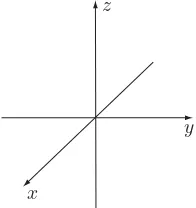
To plot a point with three coordinates the steps are just a bit more complicated. Let’s plot the point(x,y,z)₌(2,3,2). First, drawthreemutually perpendicular axes. You will immediately notice that this is impossible to do on a sheet of paper. The best you can do is two perpendicular axes, and a third at some angle to the other two (see Figure 1-1). With practice you will start to see this third axis as a perspective rendition of a line coming out of the page. When viewed this way it will seem like it is perpendicular.

Notice the way in which we labeled the axes in Figure 1-1. This is a convention, i.e., something that mathematicians have just agreed to always do. The way to remember it is by the right hand rule. What you want is to be able to position your right hand so that your thumb is pointing along the z-axis and your other ﬁngers sweep from the x-axis to they-axis when you make a ﬁst. If the axes are labeled consistent with this then we say you are using aright handed coordinate system.

OK, let’s now plot the point (2,3,2). First, locate a point 2 units from the origin on the x-axis. Now picture a planewhich goes through this point, and is perpendicular to thex-axis. Repeat this for a point 3 units from the origin on the

y-axis, and a point 2 units from the origin on thez-axis. Finally, the point(2,3,2)

is at the intersection of the three planes you are picturing.

(20)

x

y z

(2,3,2)

Figure 1-2 Plotting the point(2,3,2)

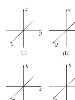
Problem 2 Which of the following coordinate systems are right handed?

(a) (b)

(c) (d)

x

x x

y y

z z

z

Problem 3 Plot the following points on one set of axes:

1. (1,1,1)

2. (1,₋1,1)

3. (₋1,1,₋1)

1.3 Introduction to Graphing

(21)

EXAMPLE 1-2

Suppose f(x,y)₌0. That is,f(x,y)is the function that always returns the number 0, no matter what values ofx andy are fed to it. The graph ofz ₌ f(x,y)₌0 is then the set of all points(x,y,z)wherez ₌0. This is just thex y-plane.

Similarly, now consider the function g(x,y)₌2. The graph is the set of all points wherez ₌g(x,y)₌2. This is a plane parallel to thex y-plane at height 2.

We ﬁrst learn to graph functions of a single variable by plotting individual points, and then playing “connect-the-dots.” Unfortunately this method doesn’t work so well in three dimensions (especially when you are trying to depict three dimensions on a piece of paper). A better strategy is to slice up the graph by various planes. This gives you several curves that you can plot. The ﬁnal graph is then obtained by assembling these curves.

The easiest slices to see are given by each of the coordinate planes. We illustrate this in the next example.

EXAMPLE 1-3

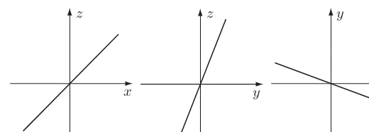
Let’s look at the function f(x,y)₌x ₊2y. To graph it we must decide which points(x,y,z)make the equationz ₌x₊2y true. Thex z-plane is the set of all points wherey ₌0. So to see the intersection of the graph of f(x,y)and thex z -plane we just sety ₌0 in the equationz ₌x₊2y. This gives the equationz₌x, which is a line of slope 1, passing through the origin.

Similarly, to see the intersection with theyz-plane we just setx ₌0. This gives us the equationz ₌2y, which is a line of slope 2, passing through the origin.

Finally, we get the intersection with the x y-plane. We must set z ₌0, which gives us the equation 0₌x₊2y. This can be rewritten asy _{= −}1₂x. We conclude this is a line with slope₋1₂.

The ﬁnal challenge is to put all of this information together on one set of axes. See Figure 1-3. We see three lines, in each of the three coordinate planes. The graph of f(x,y)is then some shape that meets each coordinate plane in the required line. Your ﬁrst guess for the shape is probably a plane. This turns out to be correct. We’ll see more evidence for it in the next section.

Problem 4 Sketch the intersections of the graphs of the following functions with each of the coordinate planes.

1. 2x₊3y

2. x2₊y

(22)

y

x

x y

z z

Figure 1-3 The intersection of the graph ofx₊2ywith each coordinate plane is a line through the origin

4. 2x2

+y2

5. x2₊_y2

6. x2

−y2

1.4 Graphing Level Curves

It’s fairly easy to plot the intersection of a graph with each coordinate plane, but this still doesn’t always give a very good idea of its shape. The next easiest thing to do is sketch some level curves. These are nothing more than the intersection of the graph with horizontal planes at various heights. We often sketch a “bird’s eye view” of these curves to get an initial feeling for the shape of a graph.

EXAMPLE 1-4

Suppose f(x,y)₌x2

+y2_{. To get the intersection of the graph with a plane at}

height 4, say, we just have to ﬁgure out which points inR3satisfyz ₌x2₊y2and

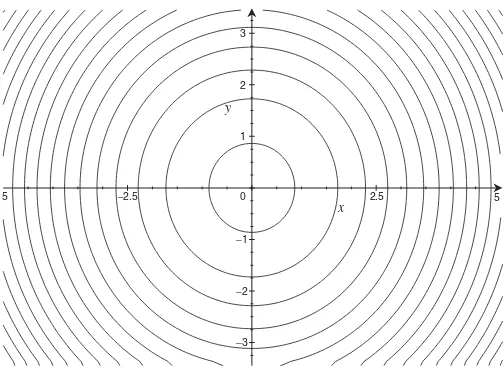
z₌4. Combining these equations gives 4₌x2₊y2, which we recognize as the equation of a circle of radius 2. We can now sketch a view of this intersection from above, and it will look like a circle in thex y-plane. See Figure 1-4.

The reason why we often draw level curves in thex y-plane as if we were looking down from above is that it is easier when there are many of them. We sketch several such curves forz ₌x2₊y2in Figure 1-5.

(23)

4

(a)

x

y

y z

(b)

Figure 1-4 (a) The intersection ofz₌x2

+y2_{with a plane at height 4. (b) A top view}

of the intersection

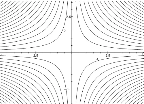
EXAMPLE 1-5

We now let f(x,y)₌x y. The intersection with the x z-plane is found by setting

y ₌0, giving us the function z ₌0. This just means the graph will include the

x-axis. Similarly, setting x ₌0 gives us z₌0 as well, so the graph will include the y-axis. Things get more interesting when we plot the level curves. Let’s set

z ₌n, wherenis an integer. Solving forythen gives usy₌ n_x. This is a hyperbola in the ﬁrst and third quadrant forn>0, and a hyperbola in the second and fourth quadrant whenn <0. We sketch this in Figure 1-8.

5 −2.5 0 2.5 5

−3

−2

−1 1 2 3

y

x

(24)

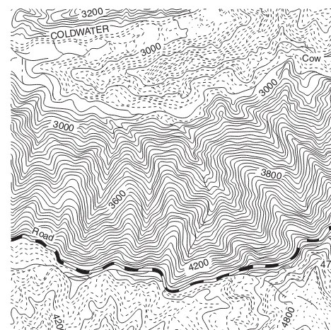
3000 3000 COLDWATER 3000 3600 4200 4200 4800 3800 3200 Cow 4785 Road

Figure 1-6 A topographic map

5645640 5040 5520 5280 548 527 541 552 551 54605280 553

553 568534

530 5400 563 562 574 581 585 586 564 553 565 543 551 525 519 519 525 568 560 569 575 581 583 564 571 57237 20 18 16 15 53 5640 5520 5400 576 573 560 5760 553 553 565 5040 5590 571 580 30 5160 565 571 570 572 579 581 580 574 577 5760 5540 5520 579 17 578 18.4 700 511 25 5040 −55 −55 −32 −36 −32 −30 −35 −33 −33 −26 −29 −38 −37 −20 −30 −28 −20 −26 −23 −48 −20 −55 −56 −23 −27 −53

−30−44 −23 −35 −36 −64 −42 −22 −33 −49 −18 −14 −29 −28 −39 −20 −23 −20 −22 −33 −18 −18 −17 −23 −23 −20 −24 −32 −17 −18 −22 −39 −14 −11 −18 −9 −35 −8 −12 −19 −48 −33 −28 −18 −17 17 −16 −34 −44 −34 −11 −45 −52 −34 −35 −20 −23 −13 −15 −14 −11 −13 −53 −37 −16 −64 −20 -20 −15 −15 −12 −44 −42 −36 −20 −30 −28 −28 −19 28 −58 5408

500 height/temp for OOZ 8 DEC 06

(25)

2.5

−2.5

5 _2.5 5

y

x

Figure 1-8 Level curves ofz₌x y

Problem 5 Sketch several level curves for the following functions.

1. 2x₊3y

2. x2₊y

3. x2₊_y2

4. x2

−y2

Problem 6 The level curves for the following functions are all circles. Describe the difference between how the circles are arranged.

1. x2₊y2

2. x2

+y2

3. _x2₊1_y2

4. sin(x2₊y2)

1.5 Putting It All Together

(26)

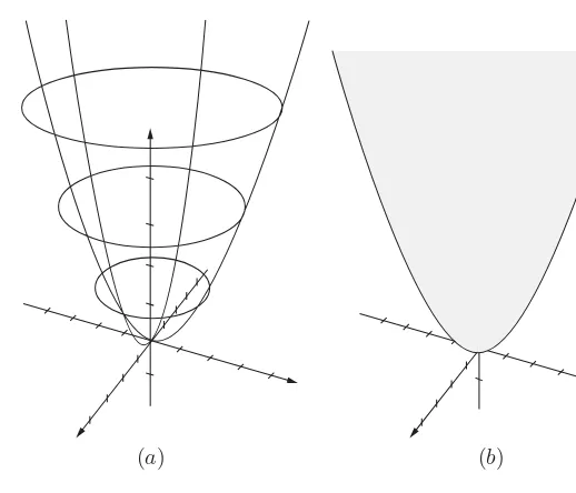
(a) (b)

Figure 1-9 Sketching the paraboloidz₌x2 +y2

EXAMPLE 1-6

Let f(x,y)₌x2₊y2. In Problem 4 you found that the intersections with the

x z- and yz-coordinate planes were parabolas. In Example 1-4 we saw that the level curves were circles. We put all of this information together in Figure 1-9(a). Figure 1-9(b) depicts the entire surface which is the graph. This ﬁgure is called a

paraboloid.

Graph sketching is complicated enough that a second example may be in order.

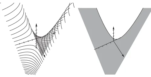
EXAMPLE 1-7

In Figure 1-10 we put together the level curves of f(x,y)₌x y, found in Example 1-5, to form its graph. The three-dimensional shape formed is called asaddle.

Problem 7 Use your answers to Problems 4 and 5 to sketch the graphs of the following functions:

1. 2x₊3y

2. x2₊y

3. 2x2₊y2

4. x2

+y2

5. x2

(27)

Figure 1-10 Several level curves ofz₌x ypiece together to form a saddle

1.6 Functions of Three Variables

There is no reason to stop at functions with two inputs and one output. We can also consider functions with three inputs and one output.

EXAMPLE 1-8

Suppose

f(x,y,z)₌x ₊x y₊yz2

Then f(1,1,1)₌3 and f(0,1,2)₌4.

To graph such a function we would need to set it equal to some fourth variable, sayw, and draw a picture in a space where there are four perpendicular axes,x,

y, z, and w. No one can visualize such a space, so we will just have to give up on graphing such functions. But all hope is not lost. We can still describe surfaces in three dimensions that are the level sets of such functions. This is not quite as good as having a graph, but it still helps give one a feel for the behavior of the function.

EXAMPLE 1-9

Suppose

f(x,y,z)₌x2₊y2₊z2

To plot level sets we set f(x,y,z)equal to various integers and sketch the surface described by the resulting equation. For example, when f(x,y,z)₌1 we have

(28)

This is precisely the equation of a sphere of radius 1. In general the level set corresponding to f(x,y,z)₌n will be a sphere of radius√n.

Problem 8 Sketch the level set corresponding to f(x,y,z)₌1for the following functions.

1. f(x,y,z)₌x2₊y2₋z2

2. f(x,y,z)₌x2₋y2₋z2

1.7 Parameterized Curves

In the previous sections of this chapter we studied functions which had multiple inputs, but one output. Here we examine the opposite scenario: functions with one input and multiple outputs. The input variable is referred to as theparameter, and is best thought of as time. For this reason we often use the variable t, so that in general such a function might look like

c(t)₌(f(t),g(t))

If we ﬁx a value oft and plot the two outputs we get a point in the plane. Ast

varies this point moves, tracing out a curve,C. We would then sayCis a curve that

isparameterized by c(t).

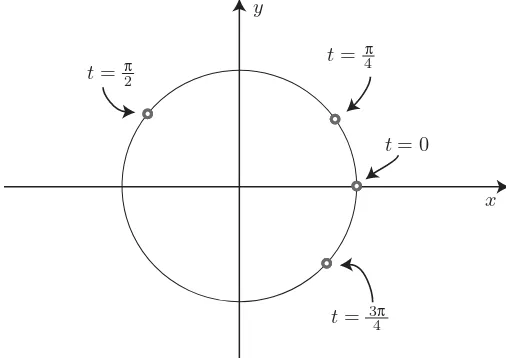
EXAMPLE 1-10

Supposec(t)₌(cost,sint). Thenc(0)₌(1,0)andcπ 2

=(0,1). If we continue to plot points we see thatc(t)traces out a circle of radius 1. Indeed, since

cos2t₊sin2t ₌1

the coordinates ofc(t)satisfyx2

+y2

=1, the equation of a circle of radius 1. In Figure 1-11 we plot the circle traced out byc(t), along with additional information which tells us what value oftyields selected point of the curve.

EXAMPLE 1-11

The functionc(t)₌(cost2_,_sin_t2₎_{also parameterizes a circle or radius 1, like the}

(29)

x y

t= 0

t= ₄

2

t=

3π

4

t=π

π

Figure 1-11 The functionc(t)₌(cost,sint)parameterizes a circle of radius 1

depicted in Figure 1-12 represents a point moving around the circle faster and faster.

EXAMPLE 1-12

Now letc(t)₌(tcost,tsint). Plotting several points shows thatc(t)parameterizes a curve that spirals out from the origin, as in Figure 1-13.

x y

t= 0

t= ₄

t= ₂

t= 3 4 π

π

(30)

x y

t= 0

t=

t=π

3π

4

π

2

t= ₄π

Figure 1-13 The functionc(t)₌(tcost,tsint)parameterizes a spiral

Parameterizations can also describe curves in three-dimensional space, as in the next example.

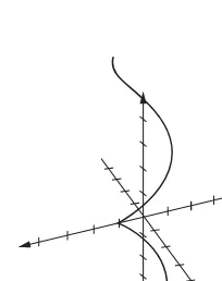
EXAMPLE 1-13

Let c(t)₌(cost,sint,t). If the third coordinate were not there then this would describe a point moving around a circle. Now as t increases the height off of the x y-plane, i.e., the z-coordinate, also increases. The result is a spiral, as in Figure 1-14.

(31)

Problem 9 Sketch the curves parameterized by the following:

1. (t,t)

2. (t,t2₎

3. (t2_,_t₎

4. (t2_,_t3₎

5. (cos 2t,sin 3t)

Problem 10 The functions given in Examples 1-10 and 1-11 parameterize the same circle in different ways. Describe the difference between the two parameterizations for negative values of t .

Problem 11 Find a parameterization for the graph of the function y₌ f(x).

Problem 12 Describe the difference between the following parameterized curves:

1. c(t)₌(cost,sint,t2)

2. c(t)₌(cost,sint,1_t)

3. c(t)₌(tcost,tsint,t)

Quiz

Problem 13

1. Determine if the coordinate system pictured is left or right handed.

y

x z

2. Let f(x,y)₌ _x2y₊₁.

a. Sketch the intersections of the graph of f(x,y) with the x y-plane, the

x z-plane, and the yz-plane.

b. Sketch the level curves for f(x,y).

c. Sketch the graph of f(x,y).

(32)

(33)

Fundamentals of

Advanced Calculus

2.1 Limits of Functions of Multiple Variables

The study of calculus begins in earnest with the concept of a limit. Without this one cannot deﬁne derivatives or integrals. Here we undertake the study of limits of functions of multiple variables.

Recall that we say lim

x→a f(x)=L if you can make f(x) stay as close to L as

you like by restrictingx to beclose enoughtoa. Just how close “close enough” is depends on how close you want f(x)to be to L.

Intuitively, if lim

x→a f(x)=Lwe think of the values of f(x)as getting closer and

closer toLas the value ofx gets closer and closer toa. A key point is that it should not matterhowthe values ofx are approachinga. For example, the function

f(x)₌ x

|x_|

(34)

does not have a limit as x _→0. This is because asx approaches 0 from the right the values of the function f(x)approach 1, while the values of f(x)approach₋1 asxapproaches 0 from the left.

The deﬁnition of limit for functions of multiple variables is very similar. We say

lim

(x,y)→(a,b) f(x,y)=L

if you can make f(x,y)stay as close to L as you like by restricting(x,y)to be

close enough to(a,b). Again, just how close “close enough” is depends on how

close you want f(x,y)to be to L.

Once again, the most useful way to think about this definition is to think of the values of f(x,y)as getting closer and closer to L as the point (x,y)gets closer and closer to the point(a,b). The difficulty is that there are now an infinite number of directions by which one can approach(a,b).

EXAMPLE 2-1

Suppose f(x,y)is given by

f(x,y)₌ x

x₊y

We consider lim

(x,y)→(0,0) f(x,y).

First, let’s see what happens as(x,y)approaches(0,0)along thex-axis. For all such points we knowy ₌0, and so

f(x,y)₌ x

x ₊y =

x

x =1

Now consider what happens as(x,y)approaches(0,0)along the y-axis. For all such points we havex ₌0, and so

f(x,y)₌ x

x ₊y =

0

y =0

We conclude the values of f(x,y) approach different numbers if we let (x,y)

approach(0,0)from different directions. Thus we say lim

(x,y)→(0,0) f(x,y)does not

exist.

(35)

same numberLdoes not necessarily mean lim

(x,y)→(a,b) f(x,y)=L. There might be

some way to approach(a,b)that you haven’t tried that gives a different number. This is the key to the deﬁnition of limit. We say the function has a limit only when the values of f(x,y)approach the same number no matter how(x,y)approaches

(a,b). We illustrate this in the next two examples.

EXAMPLE 2-2

Suppose f(x,y)is given by

f(x,y)₌ x y

x2₊_y2

As we let(x,y)approach(0,0)along thex-axis (wherey₌0) we have

f(x,y)₌ x y

x2₊_y2 =

0

x2 =0

Similarly, as we let(x,y)approach(0,0)along they-axis (wherex ₌0) we have

f(x,y)₌ x y

x2

+y2 =

0

y2 =0

But if we let(x,y)approach(0,0)along the line y ₌x we have

f(x,y)₌ x y

x2₊_y2 =

x2

2x2 =

1 2

So once again we ﬁnd lim

(x,y)→(0,0) f(x,y)does not exist.

Our third example is the trickiest.

EXAMPLE 2-3

Let

f(x,y)₌ x

2_y

x4

+y2

As(x,y)approaches(0,0)along thex-axis (wherey ₌0) we have

f(x,y)₌ x

2_y

x4₊_y2 =

0

(36)

As(x,y)approaches(0,0)along they-axis (wherex ₌0) we have

f(x,y)₌ x

2_y

x4₊_y2 =

0

y2 =0

If we approach(0,0)along the line y₌x we get

f(x,y)₌ x

2_y

x4

+y2 =

x3 x4

+x2 =

x x2

+1

Asx approaches 0 we have

lim

x→0

x

x2₊₁ =0

So far it is looking like perhaps

lim

(x,y)→(0,0)

x2y

x4₊_y2 =0

since, as(x,y)approaches(0,0)along thex-axis, they-axis, and the liney ₌x, the values of f(x,y)approach 0. But what happens if we let(x,y)approach(0,0)

along thecurve y ₌x2? In this case

f(x,y)₌ x

2_y

x4

+y2 =

x4 x4

+x4 =

1 2

We can evaluate the limit of this function asxapproaches 0 by dividing the numer-ator and denominnumer-ator byx4.

lim

x→0

x4

x2₊_x4 =_xlim_→₀

1

1 x2 +1

=1

So again the limit does not exist.

Problem 14 Show that the following limits do not exist:

1. lim

(x,y)→(0,0) x2

x2₊_y3

2. lim

(x,y)→(0,0) x2_y

x3

+y3

3. lim

(x,y)→(0,0) x+y

√

x2₊_y2

4. lim

(x,y)→(0,0) x2_y2

(37)

2.2 Continuity

We say a function f(x,y)iscontinuousat(a,b)if its limit as (x,y)approaches

(a,b)equals its value there. In symbols we write lim

(x,y)→(a,b) f(x,y)= f(a,b)

Most functions you can easily write down are continuous at every point of their domain. Hence, what you want to avoid are points outside of the domain, where you may have

1. Division by zero.

2. Square roots of negatives. 3. Logs of nonpositive numbers. 4. Tangents of odd multiples of π₂.

In each of these situations the function does not even exist, in which case it is certainly not continuous. But even if the function exists it may not have a limit. And even if the function exists, and the limits exist, they may not be equal.

EXAMPLE 2-4

Suppose

f(x,y)₌ x+y

x2

+y2

There is no zero in the denominator when(x,y)₌(1,1), so f(x,y)is contin-uous at(1,1).

EXAMPLE 2-5

Evaluate

lim

(x,y)→(0,0)

x2y3 x2

+y2

+1

There are no values ofx andythat will make the denominator 0, so the function is continuous everywhere. Since the value of a continuous function equals its limit, we can evaluate the above simply by plugging in(0,0).

lim

(x,y)→(0,0)

x2y3 x2

+y2

+1 =

(38)

Problem 15 Find the domain of the following functions:

1. x_x+₋y_y

2. y₋x2

3. ln(y₋x)√x ₋y

Problem 16 Consider the function

f(x,y)₌

x2

+y2

sin(x2₊_y2₎ (x,y)=(0,0)

1 (x,y)₌(0,0)

Is f(x,y)continuous at(0,0)?

Quiz

Problem 17

1. Show that the function

f(x,y)₌ xsiny

x2₊_y2

does not have a limit as(x,y)_→(0,0).

2. Is the function

f(x,y)₌

x+y

x+y (x,y)=(0,0)

1 (x,y)₌(0,0)

continuous at(0,0)?

3. Find the domain of the function

f(x,y)₌ln 1

(39)

Derivatives

3.1 Partial Derivatives

What shall we mean by thederivativeof f(x,y)at a point(x0,y0)? Just as in one

variable calculus, the answer is the slope of a tangent line. The problem with this is that there are multiple tangent lines one can draw to the graph ofz₌ f(x,y)at any given point. Which one shall we pick to represent the derivative? The answer is another question: “Whichderivative?” We will see that at any given point there are lots of possible derivatives; one for each tangent line.

Another way to think about this is as follows. Suppose we are at the point(x0,y0)

and we start moving. While we do this we keep track of the quantity f(x,y). The rate of change that we observe is the derivative, but the answer may depend on which direction we are traveling.

Suppose, for example, that we are observing the function f(x,y)₌x2y, while moving through the point(1,1)with unit speed. Suppose further that we are travel-ing parallel to thex-axis, so that oury-coordinate is always one. We would like to know the observed rate of change of f(x,y). Since they-coordinate is always one

(40)

the values of f(x,y)that we observe are always determined by ourx-coordinate:

f(x,1)₌x2. The rate of change of this function is given by its derivative: 2x. Finally, whenx ₌1 this is the number 2.

The above is a particularly easy computation. Given any function, if you are traveling in a direction which is parallel to the x-axis then your y-coordinate is ﬁxed. Plugging this number in fory then gives a function of justx, which we can differentiate. Here’s another example.

EXAMPLE 3-1

We compute the rate of change of f(x,y)₌x3y3 at the point (1,2), when we are traveling parallel to the x-axis. During our travels the value of y stays ﬁxed at 2. Hence, the values of the function we are observing are determined by our

x-coordinate: f(x,2)₌8x3.The derivative of this function is then 24x2, which takes on the value 24 whenx is one.

What if we wanted to repeat our computations, with different values of y? It would be helpful to keep the letter “y” in our computations, and plug in the value at the very end. Notice that when we plugged in a number foryit became a constant, and was treated as such when we differentiated with respect tox. If we leave the lettery in our computations we can still treat it as a constant.

EXAMPLE 3-2

Let f(x,y)₌x₊x y₊y2_{. We wish to treat} _y _{as a constant, just as if we had}

plugged in a number for it, and take the derivative with respect tox. Recall that the derivative of a sum of functions is the sum of the derivatives. So we will discuss the derivatives of each of the terms ofx ₊x y₊y2individually.

There is no occurrence ofyin the ﬁrst term, so it is particularly easy. Its derivative is just one.

The second term is a little trickier. Since we are treatingyas a constant this is of the formconst_·x. The derivative of such a function is justconst. So the derivative ofx yis justy.

Finally, the quantity y2is also a constant. The derivative of a constant is zero. Hence our answer is 1₊y.

(41)

variable, every other letter is a constant, and we differentiate. Similarly, the notation

∂f

∂y is thepartial derivative with respect to y.

EXAMPLE 3-3

Again we let f(x,y)₌x₊x y₊y2_{. We compute}

∂f

∂y =x+2y

There are various other ways to think of partial derivatives that are useful. One is completely algebraic. Recall that the derivative with respect to x of a function

f(x)of one variable is deﬁned as the limit

df

dx =limx_→0

f(x₊x)₋ f(x)

x

The partial with respect to x is deﬁned similarly. Just remember that y is kept constant, so that f(x,y)really becomes a function of just x. We then apply the above deﬁnition to get:

∂f

∂x =limx→0

f(x₊x,y)₋ f(x,y)

x

The partial with respect toyis deﬁned similarly

∂f

∂y =limy→0

f(x,y₊y)₋ f(x,y)

y

There is yet another way to think about the partial derivative. We began this section by claiming that the derivative will still represent the slope of a tangent line. In the following ﬁgure we see the graph of an equationz ₌ f(x,y). Through the point (x0,y0) in the xy-plane there is also drawn a vertical plane parallel to

the xz-plane. The intersection of this vertical plane with the graph is a curve. The slope of the tangent line to this curve is exactly the value of the partial derivative with respect to x at(x0,y0). To see the partial derivative with respect

to y we would have a similar picture, where the vertical plane is parallel to the

(42)

x

y z

(x0, y0)

Slope= (x0,y0) ∂f

∂x

Problem 18 Compute ∂_∂f_x(2,3)and∂_∂f_y(2,3)for the following functions.

1. x₊xy

2. xlny

3. x√xy

Problem 19 Compute ∂_∂f_x(x,y)and∂_∂f_y(x,y)for the following functions. 1. x2_y3

2. x_y

Problem 20 For the function f(x,y)_{= −}x ₊x y2₋y2ﬁnd all places where both

∂f ∂x and

∂f

∂y are zero.

3.2 Composition and the Chain Rule

3.2.1 COMPOSITION WITH PARAMETERIZED CURVES

(43)

a function f(x,y). The result is the composition f(φ (t)). Notice that only one number goes in to this function, and only one number comes out.

EXAMPLE 3-4

Let f(x,y)₌x2₊y2. Letφ (t)₌(tcost,tsint). Then

f(φ (t))₌ f(tcost,tsint)₌t2cos2t₊t2sin2t₌t2

There are various ways to visualize the composition. One is to imagine the graph of z₌ f(x,y) in three dimensions. Then draw the parameterized curveφ (t)in thex y-plane, and imagine a vertical piece of paper curled up so that it sits on this curve. Now mark where the paper intersects the graph of f(x,y), and unroll it. The result is the graph of f(φ (t)).

f(x,y) _f(f

(

t

))

f(t)

t

Unroll

Since f(φ (t))is a function of one variable we can talk about its derivative just as if we were in a ﬁrst term calculus class. But what we want to do here is relate it to the derivatives of f(x,y),x(t), and y(t). The formula we end up with is the multivariable calculus version of the “chain rule”

d

dtf(φ (t))=

∂f

∂x dx

dt +

∂f

∂y dy

dt

EXAMPLE 3-5

Let f(x,y)andφ (t)be deﬁned as in the previous example. We wish to compute

d

dt f(φ (t))whent= π

6. Note ﬁrst that

φ

π

6

=

√

3π

12 ,

π

(44)

To use the chain rule we must compute the partial derivatives of f(x,y) at this point. First note that

∂f

∂x(x,y)=2x, and

∂f

∂y(x,y)=2y

Thus, ∂f ∂x √ 3π 12 , π 12 = √ 3π

6 , and

∂f ∂y √ 3π 12 , π 12 = π 6

We also need the derivatives ofx(t)andy(t)whent ₌ π₆.

x′(t)₌cost₋tsint, and

y′(t)₌sint₊tcost

Thus, x′ π 6 = √ 3 2 − π

12, and

y′

π

6

= 1₂ +

√

3π

12

Finally, we have

d dt f φπ 6 = ∂f

∂x d x dt + ∂f ∂y d y dt = √ 3π 6 √ 3 2 − π 12 + π 6 1 2 + √ 3π 12

= π₃

(45)

muchfaster directly. We know from the previous example that f(φ (t))₌t2. So the derivative function is 2t. Plugging int ₌ π₆ then immediately gives(2)π₆₌ π₃.

Problem 21 Letφ (t)₌(2t,t2). Suppose you don’t know what f(x,y)is, but you know _∂∂_xf(2,1)₌6and _∂∂_yf(2,1)_{= −}1. Compute _dtd f(φ (1)).

Problem 22 Suppose you don’t know whatφ (t)₌(x(t),y(t)) is, but you know

φ (2)₌(1,3), x′₍₂₎_{= −}₂_, _and _y′₍₂₎₌₁_. _Let _f₍_x_,_y₎₌_x2_y. _Compute

d

dt f(φ (2)).

3.2.2 COMPOSITION OF FUNCTIONS OF MULTIPLE

VARIABLES

We now look at the idea of composition with more complicated types of functions, as in our next example.

EXAMPLE 3-6

Letx(u, v)₌uvandy(u, v)₌u2₊v2. Suppose f(x,y)₌x₊y. Then we may form the composition f(x(u, v),y(u, v))as follows.

f(x(u, v),y(u, v))₌x(u, v)₊y(u, v)₌uv₊u2₊v2

Notice that the result is a function whose input is a pair of numbers,uandv, and whose output is a single number. Hence, we may talk about the partial derivatives, with respect tou andv, of the function given by composition. The result is given by another variant of the chain rule. As in the previous example, we will begin with the functionsx(u, v),y(u, v), and f(x,y). The following formulas give the partial derivatives of the composition f(x(u, v),y(u, v)).

∂f

∂u =

∂f

∂x

∂u +

∂f

∂y

∂u

∂f

∂v = ∂f

∂x

∂v + ∂f

∂y

∂v

At this point it is mathematically meaningless to think of terms like “∂x” as entities in themselves that can be canceled, but thinking this way may help you remember the above formulas. Note that the formula for the partial derivative of f

(46)

EXAMPLE 3-7

Let f(x,y)₌x2₊x y. Suppose we don’t know x(u, v)or y(u, v), but we know

x(1,2)₌3,y(1,3)_{= −}2,_∂∂_ux(1,2)_{= −}1, and ∂_∂_uy(1,2)₌5. Then we may use the chain rule to compute ∂_∂_uf(1,2). To do this we will need to know ∂_∂f_x and ∂_∂_yf at the point(x(1,2),y(1,2))₌(3,₋2).

∂f

∂x(3,−2)=(2)(3)+(−2)=4,

∂f

∂y(3,−2)=3

We now employ the chain rule:

∂f

∂u =

∂f

∂x

∂u +

∂f

∂y

∂u

=(4)(₋1)₊(3)(5)

=11

Problem 23 The following table lists values for a function f(x,y)and its partial derivatives.

(x,y) f(x,y) ∂_∂_xf ∂_∂f_y (1,1) ₋3 ₋2 2

(1,2) 5 1 1

(2,1) 2 0 7

(2,5) ₋1 2 3

(2,3) 11 1 ₋1

(3,2) 2 1 0

Let x(u, v)₌uvand y(u, v)₌u₊v2. Find the following partial derivatives at

the indicated points.

1. ∂_∂_uf at(u, v)₌(1,2)

2. ∂_∂vf at(u, v)₌(2,1)

Problem 24 Let f(x,y)₌sin(x₊y), x(u, v)₌u₊v, and y(u, v)₌u₋v.

Find the following quantities when(u, v)₌(π₂, π ).

1. f(x,y)

2. ∂_∂_uf

(47)

3.3 Second Partials

In the previous sections we saw that the partial derivatives of a function f(x,y)are also functions of x andy. We can therefore take the derivative again with respect to either variable.

EXAMPLE 3-8

Let f(x,y)₌x2y3. The partial derivatives are _∂∂_xf ₌2x y3 and _∂∂_yf ₌3x2y2. We can take the partial derivative again of both of these functions with respect to either variable: ∂ ∂x ∂f ∂x

=2y3, ∂ ∂y

∂f

∂x

=6x y2

∂ ∂x ∂f ∂y

=6x y2, ∂ ∂y

∂f

∂y

=6x2y

As is customary, we adopt the following shorthand notations for the second derivatives: ∂ ∂x ∂f ∂x = ∂ 2_f

∂x2,

∂ ∂y ∂f ∂x = ∂ 2_f

∂y∂x

∂ ∂x ∂f ∂y = ∂ 2_f

∂x∂y,

∂ ∂y ∂f ∂y = ∂ 2_f

∂y2

The quantities _∂∂_y2_∂f_x and _∂∂_x2_∂f_y are called themixed partials. The above example illustrates an amazing fact: Under reasonable conditions the mixed partials are always equal! The “reasonable conditions” are only that the mixed partials exist and are themselves continuous functions. The proof of this goes back to the limit deﬁnition of the partial derivative.

Problem 25 Find all second partial derivatives of the following functions.

1. f(x,y)₌x y

2. f(x,y)₌x2

−y2

(48)

Quiz

Problem 26 Let f(x,y)₌x2y₊x3y2. 1. Find∂_∂_xf and ∂_∂_yf.

2. Ifφ (t)₌(t2_,_t

−1), then what is f(φ (t))?

3. Suppose you don’t know whatψ (t)₌(x(t),y(t))is, but you knowψ (2)₌

(1,1), d x_dt(2)₌3, and d y_dt(2)₌1. Find the derivative of f(ψ (t)) when

t ₌2.

4. Suppose x and y are functions of u andv, x(u, v)₌u2₊v, and y(1,1)₌1.

(49)

Integration

4.1 Integrals over Rectangular Domains

The integral of a function of one variable gives the area under the graph and above an interval on the x-axis called the domain of integration. For functions of two variables the graph is a surface. We will interpret the act of integration as that of ﬁnding the volume below the surface, and above some region in the x y-plane. Eventually, we will examine how to do this with very general-shaped regions. We begin by looking at rectangles.

x y

R

(a,b)

LetRbe the region of thex y-plane pictured above. Suppose we want to ﬁnd the volume of the region inR3_{which sits above}_R_{, and below the graph of}_z

= f(x,y), as in the following ﬁgure. We do this by following these steps.

(50)

x

y z

z=f(x,y)

1. Begin by choosing a grid of points_{(xi,yj)}inR, so that the horizontal and

vertical spacings between adjacent points arex andy, respectively. 2. Connect these grid points to break up Rinto rectangles. Note that the area

of each rectangle isxy.

x y

(xi,yj)

∆x

∆y

3. We now draw a box of height f(xi,yj)above each such rectangle to get a

ﬁgure which approximates the desired volume. The volume of each box is its length_×width_×height, which is f(xi,yj)xy.

x

y z

(51)

4. We now add up the volumes of all of these boxes to obtain the quantity

j

i

f(xi,yj)xy

5. Finally, we repeat this process indeﬁnitely, each time using a grid withxand

ysmaller and smaller. The corresponding ﬁgures that we get approximate the desired volume more and more. In the limit we get what we’re after, which we denote as

R

f(x,y)dx dy:

R

f(x,y)dx dy₌ lim

y→0limx→0

j

i

f(xi,yj)xy

Basic properties of summation and limits allow us to rearrange the above equation as follows:

R

f(x,y)dx dy₌ lim

y→0

j

lim

x→0

i

f(xi,yj)x

y

The quantity in the brackets lim

x→0

i

f(xi,yj)x is exactly the deﬁnition of

what you get from f(x,y) when you ﬁx y and integrate x, as in the following example.

EXAMPLE 4-1

Let f(x,y)₌x2₊y3. If we ﬁxy ₌3 then this is the function f(x)₌x2₊27. We may now integrate this function over some range of values ofx, such as [0,2]:

lim

x→0

i

f(xi,yj)x =

2

0

x2₊27dx₌ 1

3x

3

+27x

2

x=0

= 8₃ +56

If we don’t substitute the value 3 fory, but we still think ofyas a constant, very little changes:

2

0

x2₊y3d x ₌ 1

3x

3

+y3x

2

x=0

= 8

3 +2y

3

(52)

this new function with respect to y. This is precisely what we are instructed to do in the limit we obtained for

R

f(x,y)dx dy.

R

f(x,y)d x d y₌ lim

y→0

j

lim

x→0

i

f(xi,yj)x

y

= lim

y→0 j ⎡ ⎣ a 0

f(x,y)dx

⎤

⎦y

= b 0 ⎡ ⎣ a 0

f(x,y)dx

⎤

⎦dy

EXAMPLE 4-2

Let f(x,y)₌xy2_{. Suppose}_Q_{is the rectangle with vertices at}₍₁_,₁₎_,₍₂_,₁₎_,₍₁_,₄₎_,

and(2,4). To ﬁnd the volume under the graph of f and above this rectangle we wish to compute

Q

xy2dx dy₌

4 1 ⎡ ⎣ 2 1

x y2dx

⎤

⎦dy

We work inside the brackets ﬁrst. To do this integral we must pretend y is a constant.

2

1

x y2dx₌ 1

2x 2 y2 2 1

=2y2₋1

2y

2

= 3₂y2

We now have

4 1 ⎡ ⎣ 2 1

xy2dx

⎤

⎦dy= 4 1 3 2y 2_dy = 1 2y 3 4 1

=32₋1 2 =

63 2

Note that in the deﬁnition of

R

f(x,y) dx dywe could have rearranged the

(53)

EXAMPLE 4-3

LetSbe the rectangle with vertices at(1,0),(2,0),(1,1), and(2,1). We integrate the function f(x,y)₌exy. We compute the integral of f(x,y)overSby doing the

integral with respect toyﬁrst:

S

eyx d x d y=

2 1 ⎡ ⎣ 1 0

eyx d y

⎤ ⎦dx = 2 1

xeyx

1

y=0 dx = 2 1

xe1x −x

dx

= −xe−x ₋e−x ₋1

2x 2 2 1

= −_e32 +

2

e −

3 2

To save space the integral b

a[

d

c f(x,y)dx]dy is often written as

b a

d

c f(x,y)dx dy.

Problem 27 Compute the following:

1. 1 0 3 2

x ₊x y2dx dy

2. 1 −1 1 0

x2y2dy dx

3. π 2 0 π 2 0

cos(x ₊y)dx dy

Problem 28 Let R be the rectangle in the x y-plane with corners at (₋1,₋1),

(₋1,0), (2,₋1), and (2,0). Find the volume below the graph of z ₌x3y and

(54)

Problem 29 Let R be the rectangle with vertices at(0,0),(1,0),(0,1), and(1,1). Find a formula for

R

xnym d x d y.

Problem 30 Let V be the volume below the graph of e−x y2, and above the rectangle

with corners at(0,0),(2,0),(0,3), and(2,3). Find the area of the intersection of

V with the vertical plane through the point(1,1)which is parallel to the x z-plane.

4.2 Integrals over Nonrectangular Domains

In the previous section we saw how to compute the volume under the graph of a function and above a rectangle. But what if we are interested in the volume which lies above a nonrectangular area? For example, suppose now that R is the region of thex y-plane that is bounded by the graph ofy₌g(x), thex-axis, and the line

x ₌1. We would like to ﬁnd the volume of the ﬁgureV which lies below the graph ofz ₌ f(x,y)and above the regionR.

x

x y

y z

z=f(x,y)

R

1

In the previous section we computed volume by breaking up the region in question into small boxes. Our strategy here is to cut it into “slabs” parallel to theyz-plane. To specify the location of each slab we must give a value ofx. Hence, the volume of each slab, calculated as an integral with respect to y, is a function ofx. Adding the slabs up is just like integrating with respect tox.

We follow these steps:

1. Choose points_{xi}in the interval [0,1].

2. Compute the area A(xi)of the intersection ofV with the planex =xi. We

do this by plugging xi in for the variable x in the function f(x,y) and

(55)

this domain. So the requisite area is given by

A(xi)= g(xi)

0

f(xi,y)d y

x

x y

y z

xi

g(xi)

1

A(xi)

3. The volume of a thin slab is then given by

A(xi)x =

g(xi)

0

f(xi,y)d yx

x

y z

(56)

4. Adding up the volumes of all of the slabs thus gives

i g(xi)

0

f(xi,y)d y x

5. Finally, the desired volume is obtained from this quantity by choosing smaller and smaller slabs. This is equivalent to taking a limit asx tends toward 0.

V ₌ lim

x→0

i g(xi)

0

f(xi,y)d yx =

1

0 g(x)

0

f(x,y)d y d x

The key to understanding this formula is the limits of integration. Each slab is parallel to they-axis. The area of the side of the slab is thus computed as an integral with respect to y. But the range of values thaty can take on depends on what the value ofx is. Hence, the limits of integration of the inner integral depend onx.

EXAMPLE 4-4

Let Rbe the region in the x y-plane bounded by the graph of y ₌x2_{, the}_x_-axis,

and the linex ₌1. We compute the volume below the graph ofz ₌x y2and above

Ras follows:

Volume₌ 1 0 x2 0

x y2d y d x

=

1

0

1 3x y

3 x2 0 d x = 1 0

x7d x

= 1

8

EXAMPLE 4-5

We now use the above ideas to compute a more complicated volume. LetQbe the region of thex y-plane bounded by the graphs ofy ₌x2_and_y

=

Adv Calculus a Self Teaching guide

Demystified

TERMS OF USE

We hope you enjoy this

CONTENTS

CHAPTER 1 Functions of Multiple Variables 1

CHAPTER 4 Integration 33

CHAPTER 7 Vectors and Gradients 69

CHAPTER 9 Vector Fields and Derivatives 125

Final Exam 175

Functions of

1.2 Three Dimensions

1.3 Introduction to Graphing

EXAMPLE 1-3

1.4 Graphing Level Curves

EXAMPLE 1-5

1.5 Putting It All Together

EXAMPLE 1-7

1.6 Functions of Three Variables

EXAMPLE 1-9

1.7 Parameterized Curves

EXAMPLE 1-10

EXAMPLE 1-11

EXAMPLE 1-13

Problem 13

Fundamentals of

EXAMPLE 2-1

EXAMPLE 2-2

2.2 Continuity

EXAMPLE 2-4

Problem 17

Derivatives

EXAMPLE 3-1

EXAMPLE 3-3

3.2 Composition and the Chain Rule

EXAMPLE 3-5

3.2.2 COMPOSITION OF FUNCTIONS OF MULTIPLE

EXAMPLE 3-7

3.3 Second Partials

Integration

EXAMPLE 4-1

EXAMPLE 4-2

EXAMPLE 4-3

4.2 Integrals over Nonrectangular Domains

EXAMPLE 4-4