Pro Spark
Streaming
The Zen of Real-time Analytics using
Apache Spark
—
Pro Spark Streaming
The Zen of Real-Time Analytics
Using Apache Spark
Zubair Nabi
Zubair Nabi
This work is subject to copyright. All rights are reserved by the Publisher, whether the whole or part of the material is concerned, specifically the rights of translation, reprinting, reuse of illustrations, recitation, broadcasting, reproduction on microfilms or in any other physical way, and transmission or information storage and retrieval, electronic adaptation, computer software, or by similar or dissimilar methodology now known or hereafter developed. Exempted from this legal reservation are brief excerpts in connection with reviews or scholarly analysis or material supplied specifically for the purpose of being entered and executed on a computer system, for exclusive use by the purchaser of the work. Duplication of this publication or parts thereof is permitted only under the provisions of the Copyright Law of the Publisher’s location, in its current version, and permission for use must always be obtained from Springer. Permissions for use may be obtained through RightsLink at the Copyright Clearance Center. Violations are liable to prosecution under the respective Copyright Law.
Trademarked names, logos, and images may appear in this book. Rather than use a trademark symbol with every occurrence of a trademarked name, logo, or image we use the names, logos, and images only in an editorial fashion and to the benefit of the trademark owner, with no intention of infringement of the trademark.
The use in this publication of trade names, trademarks, service marks, and similar terms, even if they are not identified as such, is not to be taken as an expression of opinion as to whether or not they are subject to proprietary rights. While the advice and information in this book are believed to be true and accurate at the date of publication, neither the authors nor the editors nor the publisher can accept any legal responsibility for any errors or omissions that may be made. The publisher makes no warranty, express or implied, with respect to the material contained herein.
Managing Director: Welmoed Spahr Acquisitions Editor: Celestin Suresh John Developmental Editor: Matthew Moodie Technical Reviewer: Lan Jiang
Editorial Board: Steve Anglin, Pramila Balen, Louise Corrigan, James DeWolf, Jonathan Gennick, Robert Hutchinson, Celestin Suresh John, Nikhil Karkal, James Markham, Susan McDermott, Matthew Moodie, Douglas Pundick, Ben Renow-Clarke, Gwenan Spearing
Coordinating Editor: Rita Fernando Copy Editor: Tiffany Taylor Compositor: SPi Global Indexer: SPi Global
Cover image designed by Freepik.com
Distributed to the book trade worldwide by Springer Science+Business Media New York, 233 Spring Street, 6th Floor, New York, NY 10013. Phone 1-800-SPRINGER, fax (201) 348-4505, e-mail [email protected] , or visit www.springer.com . Apress Media, LLC is a California LLC and the sole member (owner) is Springer Science + Business Media Finance Inc (SSBM Finance Inc). SSBM Finance Inc is a Delaware corporation.
For information on translations, please e-mail [email protected] , or visit www.apress.com .
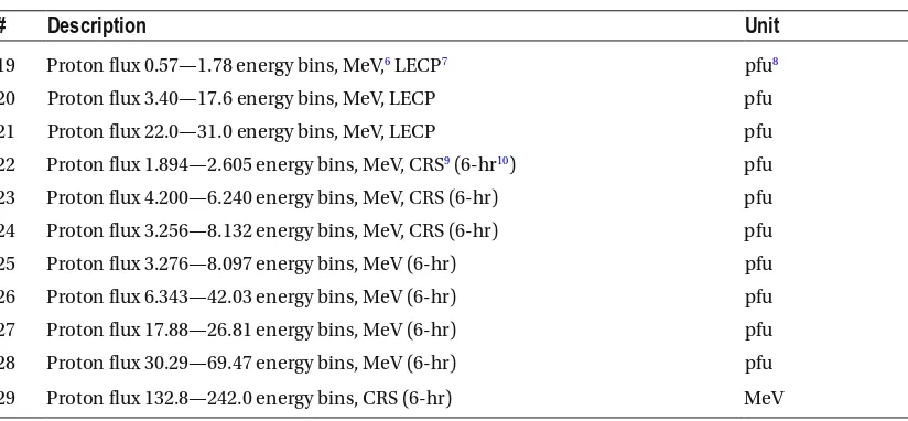
Apress and friends of ED books may be purchased in bulk for academic, corporate, or promotional use. eBook versions and licenses are also available for most titles. For more information, reference our Special Bulk Sales–eBook Licensing web page at www.apress.com/bulk-sales .
Any source code or other supplementary materials referenced by the author in this text is available to readers at www.apress.com . For detailed information about how to locate your book’s source code, go to
Contents at a Glance
About the Author ... xiii
About the Technical Reviewer ...xv
Acknowledgments ...xvii
Introduction ...xix
■
Chapter 1: The Hitchhiker’s Guide to Big Data ... 1
■
Chapter 2: Introduction to Spark ... 9
■
Chapter 3: DStreams: Real-Time RDDs ... 29
■
Chapter 4: High-Velocity Streams: Parallelism and Other Stories ... 51
■
Chapter 5: Real-Time Route 66: Linking External Data Sources ... 69
■
Chapter 6: The Art of Side Effects ... 99
■
Chapter 7: Getting Ready for Prime Time ... 125
■
Chapter 8: Real-Time ETL and Analytics Magic ... 151
■
Chapter 9: Machine Learning at Scale ... 177
■
Chapter 10: Of Clouds, Lambdas, and Pythons ... 199
Contents
About the Author ... xiii
About the Technical Reviewer ...xv
Acknowledgments ...xvii
Introduction ...xix
■
Chapter 1: The Hitchhiker’s Guide to Big Data ... 1
Before Spark ... 1
The Era of Web 2.0 ... 2
Sensors, Sensors Everywhere ... 6
Spark Streaming: At the Intersection of MapReduce and CEP ... 8
■
Chapter 2: Introduction to Spark ... 9
Installation ... 10
Execution ... 11
Standalone Cluster ... 11
YARN ... 12
First Application ... 12
Build ... 14
Execution ... 15
SparkContext ... 17
Creation of RDDs ... 17
Handling Dependencies ... 18
Creating Shared Variables ... 19
RDD ... 20
Persistence ... 21
Transformations ... 22
Actions ... 26
Summary ... 27
■
Chapter 3: DStreams: Real-Time RDDs ... 29
From Continuous to Discretized Streams ... 29
First Streaming Application ... 30
Build and Execution ... 32
StreamingContext ... 32
DStreams ... 34
The Anatomy of a Spark Streaming Application ... 36
Transformations ... 40
Summary ... 50
■
Chapter 4: High-Velocity Streams: Parallelism and Other Stories ... 51
One Giant Leap for Streaming Data ... 51
Parallelism... 53
Worker ... 53
Executor ... 54
Task ... 56
Batch Intervals ... 59
Scheduling ... 60
Inter-application Scheduling ... 60
Batch Scheduling ... 61
Inter-job Scheduling ... 61
One Action, One Job... 61
Memory ... 63
Serialization ... 63
Compression ... 65
Every Day I’m Shuffl ing ... 66
Early Projection and Filtering ... 66
Always Use a Combiner ... 66
Generous Parallelism ... 66
File Consolidation ... 66
More Memory ... 66
Summary ... 67
■
Chapter 5: Real-Time Route 66: Linking External Data Sources ... 69
Smarter Cities, Smarter Planet, Smarter Everything ... 69
ReceiverInputDStream ... 71
Sockets ... 72
MQTT ... 80
Flume ... 84
Push-Based Flume Ingestion ... 85
Pull-Based Flume Ingestion ... 86
Kafka ... 86
Receiver-Based Kafka Consumer ... 89
Direct Kafka Consumer ... 91
Twitter ... 92
Block Interval ... 93
Custom Receiver ... 93
HttpInputDStream ... 94
Summary ... 97
■
Chapter 6: The Art of Side Effects ... 99
Taking Stock of the Stock Market ... 99
foreachRDD ... 101
Per-Record Connection ... 103
Static Connection ... 104
Lazy Static Connection ... 105
Static Connection Pool ... 106
Scalable Streaming Storage ... 108
HBase ... 108
Stock Market Dashboard ... 110
SparkOnHBase ... 112
Cassandra ... 113
Spark Cassandra Connector ... 115
Global State ... 116
Static Variables ... 116
updateStateByKey() ... 118
Accumulators ... 119
External Solutions ... 121
Summary ... 123
■
Chapter 7: Getting Ready for Prime Time ... 125
Every Click Counts ... 125
Tachyon (Alluxio) ... 126
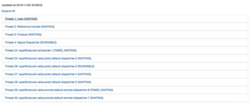
Spark Web UI ... 128
Historical Analysis ... 142
RESTful Metrics ... 142
Logging... 143
External Metrics ... 144
System Metrics ... 146
Monitoring and Alerting ... 147
■
Chapter 8: Real-Time ETL and Analytics Magic ... 151
The Power of Transaction Data Records ... 151
First Streaming Spark SQL Application ... 153
SQLContext ... 155
Data Frame Creation ... 155
SQL Execution ... 158
Confi guration ... 158
User-Defi ned Functions ... 159
Catalyst: Query Execution and Optimization ... 160
HiveContext... 160
Data Frame ... 161
Types ... 162
Query Transformations ... 162
Actions ... 168
RDD Operations ... 170
Persistence ... 170
Best Practices ... 170
SparkR ... 170
First SparkR Application ... 171
Execution ... 172
Streaming SparkR ... 173
Summary ... 175
■
Chapter 9: Machine Learning at Scale ... 177
Sensor Data Storm ... 177
Streaming MLlib Application ... 179
MLlib... 182
Data Types ... 182
Statistical Analysis... 184
Feature Selection and Extraction ... 186
Chi-Square Selection ... 186
Principal Component Analysis ... 187
Learning Algorithms ... 187
Classifi cation ... 188
Clustering ... 189
Recommendation Systems ... 190
Frequent Pattern Mining ... 193
Streaming ML Pipeline Application... 194
ML ... 196
Cross-Validation of Pipelines ... 197
Summary ... 198
■
Chapter 10: Of Clouds, Lambdas, and Pythons ... 199
A Good Review Is Worth a Thousand Ads ... 200
Google Dataproc ... 200
First Spark on Dataproc Application ... 205
PySpark ... 212
Lambda Architecture ... 214
Lambda Architecture using Spark Streaming on Google Cloud Platform ... 215
Streaming Graph Analytics ... 222
Summary ... 225
About the Author
Zubair Nabi is one of the very few computer scientists who have solved Big Data problems in all three domains: academia, research, and industry. He currently works at Qubit, a London-based start up backed by Goldman Sachs, Accel Partners, Salesforce Ventures, and Balderton Capital, which helps retailers understand their customers and provide personalized customer experience, and which has a rapidly growing client base that includes Staples, Emirates, Thomas Cook, and Topshop. Prior to Qubit, he was a researcher at IBM Research, where he worked at the intersection of Big Data systems and analytics to solve real-world problems in the telecommunication, electricity, and urban dynamics space.
Zubair’s work has been featured in MIT Technology Review , SciDev , CNET , and Asian Scientist , and on Swedish National Radio, among others. He has authored more than 20 research papers, published by some of the top publication venues in computer science including USENIX Middleware, ECML PKDD, and IEEE BigData; and he also has a number of patents to his credit.
About the Technical Reviewer
Lan Jiang is a senior solutions consultant from Cloudera. He is an enterprise architect with more than 15 years of consulting experience, and he has a strong track record of delivering IT architecture solutions for Fortune 500 customers. He is passionate about new technology such as Big Data and cloud computing. Lan worked as a consultant for Oracle, was CTO for Infoble, was a managing partner for PARSE Consulting, and was a managing partner for InSemble Inc. prior to joining Cloudera. He earned his MBA from Northern Illinois University, his master’s in computer science from University of Illinois at Chicago, and his bachelor’s degree in biochemistry from Fudan University.
Acknowledgments
This book would not have been possible without the constant support, encouragement, and input of a number of people. First and foremost, Ammi and Sumaira deserve my neverending gratitude for being the bedrocks of my existence and for their immeasurable love and support, which helped me thrive under a mountain of stress.
Writing a book is definitely a labor of love, and my friends Devyani, Faizan, Natasha, Omer, and Qasim are the reason I was able to conquer this labor without flinching.
I cannot thank Lan Jiang enough for his meticulous attention to detail and for the technical rigour and depth that he brought to this book. Mobin Javed deserves a special mention for reviewing initial drafts of the first few chapters and for general discussions regarding open and public data.
Introduction
One million Uber rides are booked every day, 10 billion hours of Netflix videos are watched every month, and $1 trillion are spent on e-commerce web sites every year. The success of these services is underpinned by Big Data and increasingly, real-time analytics. Real-time analytics enable practitioners to put their fingers on the pulse of consumers and incorporate their wants into critical business decisions. We have only touched the tip of the iceberg so far. Fifty billion devices will be connected to the Internet within the next decade, from smartphones, desktops, and cars to jet engines, refrigerators, and even your kitchen sink. The future is data, and it is becoming increasingly real-time. Now is the right time to ride that wave, and this book will turn you into a pro.
The low-latency stipulation of streaming applications, along with requirements they share with general Big Data systems—scalability, fault-tolerance, and reliability—have led to a new breed of real-time computation. At the vanguard of this movement is Spark Streaming, which treats stream processing as discrete microbatch processing. This enables low-latency computation while retaining the scalability and fault-tolerance properties of Spark along with its simple programming model. In addition, this gives streaming applications access to the wider ecosystem of Spark libraries including Spark SQL, MLlib, SparkR, and GraphX. Moreover, programmers can blend stream processing with batch processing to create applications that use data at rest as well as data in motion. Finally, these applications can use out-of-the-box integrations with other systems such as Kafka, Flume, HBase, and Cassandra. All of these features have turned Spark Streaming into the Swiss Army Knife of real-time Big Data processing. Throughout this book, you will exercise this knife to carve up problems from a number of domains and industries.
This book takes a use-case-first approach: each chapter is dedicated to a particular industry vertical. Real-time Big Data problems from that field are used to drive the discussion and illustrate concepts from Spark Streaming and stream processing in general. Going a step further, a publicly available dataset from that field is used to implement real-world applications in each chapter. In addition, all snippets of code are ready to be executed. To simplify this process, the code is available online, both on GitHub 1 and on the
publisher’s web site. Everything in this book is real: real examples, real applications, real data, and real code. The best way to follow the flow of the book is to set up an environment, download the data, and run the applications as you go along. This will give you a taste for these real-world problems and their solutions.
These are exciting times for Spark Streaming and Spark in general. Spark has become the largest open source Big Data processing project in the world, with more than 750 contributors who represent more than 200 organizations. The Spark codebase is rapidly evolving, with almost daily performance improvements and feature additions. For instance, Project Tungsten (first cut in Spark 1.4) has improved the performance of the underlying engine by many orders of magnitude. When I first started writing the book, the latest version of Spark was 1.4. Since then, there have been two more major releases of Spark (1.5 and 1.6). The changes in these releases have included native memory management, more algorithms in MLlib, support for deep learning via TensorFlow, the Dataset API, and session management. On the Spark Streaming front, two major features have been added: mapWithState to maintain state across batches and using back pressure to throttle the input rate in case of queue buildup. 2 In addition, managed Spark cloud offerings from the likes of Google, Databricks, and
1
© Zubair Nabi 2016The Hitchhiker’s Guide to Big Data
From a little spark may burst a flame.
—Dante
By the time you get to the end of this paragraph, you will have processed 1,700 bytes of data. This number will grow to 500,000 bytes by the end of this book. Taking that as the average size of a book and multiplying it by the total number of books in the world (according to a Google estimate, there were 130 million books in the world in 2010 1 ) gives 65 TB. That is a staggering amount of data that would require 130 standard, off-the-shelf 500 GB hard drives to store.
Now imagine you are a book publisher and you want to translate all of these books into multiple languages (for simplicity, let’s assume all these books are in English). You would like to translate each line as soon as it is written by the author—that is, you want to perform the translation in real time using a stream of lines rather than waiting for the book to be finished. The average number of characters or bytes per line is 80 (this also includes spaces). Let’s assume the author of each book can churn out 4 lines per minute (320 bytes per minute), and all the authors are writing concurrently and nonstop. Across the entire 130 million-book corpus, the figure is 41,600,000,000 bytes, or 41.6 GB per minute. This is well beyond the processing capabilities of a single machine and requires a multi-node cluster. Atop this cluster, you also need a real-time data-processing framework to run your translation application. Enter Spark Streaming. Appropriately, this book will teach you to architect and implement applications that can process data at scale and at line-rate. Before discussing Spark Streaming, it is important to first trace the origin and evolution of Big Data systems in general and Spark in particular. This chapter does just that.
Before Spark
Two major trends were the precursors to today’s Big Data processing systems, such as Hadoop and Spark: Web 2.0 applications, for instance, social networks and blogs; and real-time sources, such as sensor networks, financial trading, and bidding. Let’s discuss each in turn.
1 Leonid Taycher, “Books of the world, stand up and be counted! All 129,864,880 of you,” Google Books Search , 2010,
http://booksearch.blogspot.com/2010/08/books-of-world-stand-up-and-be-counted.html .
The Era of Web 2.0
The new millennium saw the rise of Web 2.0 applications , which revolved around user-generated content. The Internet went from hosting static content to content that was dynamic, with the end user in the driving seat. In a matter of months, social networks, photo sharing, media streaming, blogs, wikis, and their ilk became ubiquitous. This resulted in an explosion in the amount of data on the Internet. To even store this data, let alone process it, an entirely different new of computing, dubbed warehouse-scale computing, 2, 3 was needed.
In this architecture, data centers made up of commodity off-the-shelf servers and network switches act as a large distributed system. To exploit economies of scale, these data centers host tens of thousands of machines under the same roof, using a common power and cooling mechanism. Due to the use of commodity hardware, failure is the norm rather than the exception. As a consequence, both the hardware topology and the software stack are designed with this as a first principle. Similarly, computation and data are load-balanced across many machines for processing and storage parallelism. For instance, Google search queries are sharded across many machines in a tree-like, divide-and-conquer fashion to ensure low latency by exploiting parallelism. 4 This data needs to be stored somewhere before any processing can take place—a role fulfilled by the relational model for more than four decades.
From SQL to NoSQL
The size, speed, and heterogeneity of this data, coupled with application requirements, forced the industry to reconsider the hitherto role of relational database-management systems as the de facto standard. The relational model, with its Atomicity, Consistency, Isolation, Durability (ACID) properties could not cater to the application requirements and the scale of the data; nor were some of its guarantees required any longer. This led to the design and wide adoption of the Basically Available, Soft state, Eventual consistency (BASE) model. The BASE model relaxed some of the ACID guarantees to prioritize availability over consistency: if multiple readers/writers access the same shared resource, their queries always go through, but the result may be inconsistent in some cases.
This trade-off was formalized by the Consistency, Availability, Partitioning (CAP) theorem. 5, 6 According to this theorem, only two of the three CAP properties can be achieved at the same time. 7 For instance, if you want availability, you must forego either consistency or tolerance to network partitioning. As discussed earlier, hardware/software failure is a given in data centers due to the use of commodity off-the-shelf hardware. For that reason, network partitioning is a common occurrence, which means storage systems must trade off either availability or consistency. Now imagine you are designing the next Facebook, and you have to make that choice. Ensuring consistency means some of your users will have to wait a few milliseconds or even seconds before they are served any content. On the other hand, if you opt for availability, these users will always be served content—but some of it may be stale. For example, a user’s Facebook newsfeed might contain posts that have been deleted. Remember, in the Web 2.0 world, the user is the main target (more users mean more revenue for your company), and the user’s attention span (and in turn patience span) is very short. 8 Based on this fact, the choice is obvious: availability over consistency.
2 IEEE Computer Society, “Web Search for a Planet: The Google Cluster Architecture,” 2003, http://static.
googleusercontent.com/media/research.google.com/en//archive/googlecluster-ieee.pdf .
3 Luiz André Barroso and Urs Hölzle, The Datacenter as a Computer: An Introduction to the Design of Warehouse-Scale
Machines (Morgan& Claypool, 2009), www.morganclaypool.com/doi/abs/ 10.2200/S00193ED1V01Y200905CAC006 .
4 Jeffrey Dean and Luiz André Barroso, “The Tail at Scale,” Commun. ACM 56, no 2 (February 2013), 74-80.
5 First described by Eric Brewer, the Chief Scientist of Inktomi, one of the earliest web giants in the 1990s.
6 Werner Vogels, “Eventually Consistent – Revisited,” All Things Distributed , 2008, www.allthingsdistributed.com/
A nice side property of eventual consistency is that applications can read/write at a much higher throughput and can also shard as well as replicate data across many machines. This is the model adopted by almost all contemporary NoSQL (as opposed to traditional SQL) data stores. In addition to higher scalability and performance, most NoSQL stores also have simpler query semantics in contrast to the somewhat restrictive SQL interface. In fact, most NoSQL stores only expose simple key/value semantics. For instance, one of the earliest NoSQL stores, Amazon’s Dynamo, was designed with Amazon’s platform requirements in mind. Under this model, only primary-key access to data, such as customer information and bestseller lists, is required; thus the relational model and SQL are overkill. Examples of popular NoSQL stores include key-value stores, such as Amazon’s DynamoDB and Redis; column-family stores, such as Google’s BigTable (and its open source version HBase) and Facebook’s Cassandra; and document stores, such as MongoDB.
MapReduce: The Swiss Army Knife of Distributed Data Processing
As early as the late 1990s, engineers at Google realized that most of the computations they performed internally had three key properties:
• Logically simple, but complexity was added by control code.
• Processed data that was distributed across many machines.
• Had divide-and-conquer semantics.
Borrowing concepts from functional programming, Google used this information to design a library for large-scale distributed computation, called MapReduce. In the MapReduce model, the user only has to provide map and reduce functions; the underlying system does all the heavy lifting in terms of scheduling, data transfer, synchronization, and fault tolerance.
In the MapReduce paradigm, the map function is invoked for each input record to produce key-value pairs. A subsequent internal groupBy and shuffle (transparent to the user) group different keys together and invoke the reduce function for each key. The reduce function simply aggregates records by key. Keys are hash-partitioned by default across reduce tasks. MapReduce uses a distributed file system, called the Google File System (GFS), for data storage. Input is typically read from GFS by the map tasks and written back to GFS at the end of the reduce phase. Based on this, GFS is designed for large, sequential, bulk reads and writes.
GFS is deployed on the same nodes as MapReduce, with one node acting as the master to keep metadata information while the rest of the nodes perform data storage on the local file system. To exploit data locality, map tasks are ideally executed on the same nodes as their input: MapReduce ships out computation closer to the data than vice versa to minimize network I/O. GFS divvies up files into chunks/blocks where each chunk is replicated n times (three by default). These chunks are then distributed across a cluster by exploiting its typical three-tier architecture. The first replica is placed on the same node if the writer is on a data node; otherwise a random data node is selected. The second and third replicas are shipped out to two distinct nodes on a different rack. Typically, the number of map tasks is equivalent to the number of chunks in the input dataset, but it can differ if the input split size is changed. The number of reduce tasks, on the other hand, is a configurable value that largely depends on the capabilities of each node.
one—registers its output; the other is killed. This optimization helps to negate hardware heterogeneity. For reduce functions, which are associative and commutative, an optional combiner can also be provided; it is applied locally to the output of each map task. In most cases, this combine function is a local version of the reduce function and helps to minimize the amount of data that needs to be shipped across the network during the shuffle phase.
Word Count a la MapReduce
To illustrate the flow of a typical MapReduce job, let’s use the canonical word-count example . The purpose of the application is to count the occurrences of each word in the input dataset. For the sake of simplicity, let’s assume that an input dataset—say, a Wikipedia dump—already resides on GFS. The following map and reduce functions (in pseudo code) achieve the logic of this application:
map(k, v):
for word in v.split(" "): emit((word, 1))
reduce(k, v): sum = 0
for count in v.iterator(): sum += count
emit(k, sum)
Here’s the high-level flow of this execution:
1. Based on the specified format of the input file (in this case, text) the MapReduce subsystem uses an input reader to read the input file from GFS line by line. For each line, it invokes the map function.
2. The first argument of the map function is the line number, and the second is the line itself in the form of a text object (say, a string). The map function splits the line at word boundaries using space characters. Then, for each word, it emits (to a component, let’s call it the collector ) the word itself and the value 1.
3. The collector maintains an in-memory buffer that it periodically spills to disk. If an optional combiner has been turned on, it invokes that on each key (word) before writing it to a file (called a spill file ). The partitioner is invoked at this point as well, to slice up the data into per-reducer partitions. In addition, the keys are sorted. Recall that if the reduce function is employed as a combiner, it needs to be associative and commutative. Addition is both, that’s why the word-count reduce can also be used as a combiner.
4. Once a configurable number of map s have completed execution, reduce tasks are scheduled. They first pull their input from map tasks (the sorted spill files created by the collector) and perform an n -way merge. After this, the user-provided reduce function is invoked for each key and its list of values.
Google internally used MapReduce for many years for a large number of applications including Inverted Index and PageRank calculations. Some of these applications were subsequently retired and reimplemented in newer frameworks, such as Pregel 9 and Dremel. 10 The engineers who worked on
MapReduce and GFS shared their creations with the rest of the world by documenting their work in the form of research papers. 11, 12 These seminal publications gave the rest of the world insight into the inner wirings of the Google engine.
Hadoop: An Elephant with Big Dreams
In 2004, Doug Cutting and Mike Cafarella, both engineers at Yahoo! who were working on the Nutch search engine, decided to employ MapReduce and GFS as the crawl and index and, storage layers for Nutch, respectively. Based on the original research papers, they reimplemented MapReduce and GFS in Java and christened the project Hadoop (Doug Cutting named it after his son’s toy elephant). Since then, Hadoop has evolved to become a top-level Apache project with thousands of industry users. In essence, Hadoop has become synonymous with Big Data processing, with a global market worth multiple billions of dollars. In addition, it has spawned an entire ecosystem of projects, including high-level languages such as Pig and FlumeJava (open source variant Crunch); structured data storage, such as Hive and HBase; and data-ingestion solutions, such as Sqoop and Flume; to name a few. Furthermore, libraries such as Mahout and Giraph use Hadoop to extend its reach to domains as diverse as machine learning and graph processing.
Although the MapReduce programming model at the heart of Hadoop lends itself to a large number of applications and paradigms, it does not naturally apply to others:
• Two-stage programming model: A particular class of applications cannot be implemented using a single MapReduce job. For example, a top-k calculation requires two MapReduce jobs: the first to work out the frequency of each word, and the second to perform the actual top-k ranking. Similarly, one instance of a PageRank algorithm also requires two MapReduce jobs: one to calculate the new page rank and one to link ranks to pages. In addition to the somewhat awkward programming model, these applications also suffer from performance degradation, because each job requires data materialization. External solutions, such as Cascading and Crunch, can be used to overcome some of these shortcomings.
• Low-level programming API: Hadoop enforces a low interface in which users have to write map and reduce functions in a general-purpose programming language such as Java, which is not the weapon of choice for most data scientists (the core users of systems like Hadoop). In addition, most data-manipulation tasks are repetitive and require the invocation of the same function multiple times across applications. For instance, filtering out a field from CSV data is a common task. Finally, stitching together a directed acyclic graph of computation for data science tasks requires writing custom code to deal with scheduling, graph construction, and end-to-end fault tolerance. To remedy this, a number of high-level languages that expose a SQL-like interface have been implemented atop Hadoop and MapReduce, including Pig, JAQL, and HiveQL.
9 Grzegorz Malewicz et al., “Pregel: A System for Large-Scale Graph Processing,” Proceedings of
SIGMOD ‘10 (ACM, 2010), 135-146.
10 Sergey Melnik et al., “Dremel: Interactive Analysis of Web-Scale Datasets, Proc. VLDB Endow 3 ,
no. 1-2 (September 2010), 330-339.
11 Jeffrey Dean and Sanjay Ghemawat, “MapReduce: Simplified Data Processing on Large Clusters,” Proceedings of
OSDI 04 6 (USENIX Association, 2004), 10.
12 Sanjay Ghemawat, Howard Gobioff, and Shun-Tak Leung, “The Google File System,” Proceedings of SOSP ‘03
• Iterative applications: Iterative applications that perform the same computation multiple times are also a bad fit for Hadoop. Many machine-learning algorithms belong to this class of applications. For example, k-means clustering in Mahout refines its centroid location in every iteration. This process continues until a
threshold of iterations or a convergence criterion is reached. It runs a driver program on the user’s local machine, which performs the convergence test and schedules iterations. This has two main limitations: the output of each iteration needs to be materialized to HDFS, and the driver program resides in the user’s local machine at an I/O cost and with weaker fault tolerance.
• Interactive analysis: Results of MapReduce jobs are available only at the end of execution. This is not viable for large datasets where the user may want to run interactive queries to first understand their semantics and distribution before running full-fledged analytics. In addition, most of the time, many queries need to be run against the same dataset. In the MapReduce world, each query runs as a separate job, and the same dataset needs to be read and loaded into memory each time.
• Strictly batch processing: Hadoop is a batch-processing system, which means its jobs expect all the input to have been materialized before processing can commence. This model is in tension with real-time data analysis, where a (potentially continuous) stream of data needs to be analyzed on the fly. Although a few attempts 13 have been made to retrofit Hadoop to cater to streaming applications, none of them have been able to gain wide traction. Instead, systems tailor-made for real-time and streaming analytics, including Storm, S4, Samza, and Spark Streaming, have been designed and employed over the last few years.
• Conflation between control and computation: Hadoop v1 by default assumes full control over a cluster and its resources. This resource hoarding prevents other systems from sharing these resources. To cater to disparate application needs and data sources, and to consolidate existing data center investments, organizations have been looking to deploy multiple systems, such as Hadoop, Storm, Hama, and so on, on the same cluster and pass data between them. Apache YARN, which separates the MapReduce computation layer from the cluster-management and -control layer in Hadoop, is one step in that direction. Apache Mesos is another similar framework that enables platform heterogeneity in the same namespace.
Sensors, Sensors Everywhere
TelegraphCQ. 18 Of these, Aurora was subsequently commercialized by StreamBase Systems 19 (later acquired by TIBCO) as StreamBase CEP, with a high-level description language called StreamSQL, running atop a low-latency dataflow engine. Other examples of commercial systems included IBM InfoSphere Streams 20 and Software AG Apama streaming analytics. 21
Widespread deployment of IoT devices and real-time Web 2.0 analytics at the end of the 2000s breathed fresh life into stream-processing systems . This time, the effort was spearheaded by the industry. The first system to emerge out of this resurgence was S4 22, 23 from Yahoo!. S4 combines the Actors model with the simplified MapReduce programming model to achieve general-purpose stream processing. Other features include completely decentralized execution (thanks to ZooKeeper, a distributed cluster-coordination system) and lossy failure. The programming model consists of processing elements connected via streams to form a graph of computation. Processing elements are executed on nodes, and communication takes place via partitioned events .
Another streaming system from the same era is Apache Samza 24 (originally developed at LinkedIn), which uses YARN for resource management and Kafka (a pub/sub-based log-queuing system) 25 for messaging. As a result, its message-ordering and -delivery guarantees depend on Kafka. Samza messages have at-least-once semantics, and ordering is guaranteed in a Kafka partition. Unlike S4, which is completely decentralized, Samza relies on an application master for management tasks, which interfaces with the YARN resource manager. Stitching together tasks using Kafka messages creates Samza jobs, which are then executed in containers obtained from YARN.
The most popular and widely used system in the Web 2.0 streaming world is Storm. 26 Originally developed at the startup BackType to support its social media analytics, it was open sourced once Twitter acquired the company. It became a top-level Apache project in late 2014 with hundreds of industry deployments. Storm applications constitute a directed acyclic graph (called a topology ) where data flows from sources (called spouts ) to output channels (standard output, external storage, and so on). Both intermediate transformations and external output are implemented via bolts . Tuple communication channels are established between tasks via named streams . A central Nimbus process handles job and resource orchestration while each worker node runs a Supervisor daemon, which executes tasks (spouts and bolts) in worker processes. Storm enables three delivery modes: at-most-once, at-least-once, and exactly-once. At-most-once is the default mode in which messages that cannot be processed are dropped. At-least-once semantics are provided by the guaranteed tuple-processing mode in which downstream operators need to acknowledge each tuple. Tuples that are not acknowledged within a configurable time duration are replayed. Finally, exactly-once semantics are ensured by Trident, which is a batch-oriented, high-level transactional abstraction atop Storm. Trident is very similar in spirit to Spark Streaming.
In the last few years, a number of cloud-hosted, fully managed streaming systems have also emerged, including Amazon’s Kinesis, 27 Microsoft’s Azure Event Hubs, 28 and Google’s Cloud Dataflow. 29 Let’s consider a brief description of Cloud Dataflow as a representative system. Cloud Dataflow under the hood employs
18 http://telegraph.cs.berkeley.edu/ .
19 www.streambase.com/ .
20 http://www-03.ibm.com/software/products/en/infosphere-streams .
21 www.softwareag.com/corporate/products/apama_webmethods/analytics/overview/default.asp .
22 Leonardo Neumeyer et al., “S4: Distributed Stream Computing Platform,” Proceedings of
MillWheel 30 and MapReduce as the processing engines and FlumeJava 31 as the programming API. MillWheel is a stream-processing system developed in house at Google, with one delineating feature: low watermark. The low watermark is a monotonically increasing timestamp signifying that all events until that timestamp have been processed. This removes the need for strict ordering of events. In addition, the underlying system ensures exactly-once semantics (in contrast to Storm, which uses a custom XOR scheme for deduplication, MillWheel uses Bloom filters). Atop this engine, FlumeJava provides a Java Collections–centric API, wherein data is abstracted in a PCollection object, which is materialized only when a transform is applied to it. Out of the box it interfaces with BigQuery, PubSub, Cloud BigTable, and many others.
Spark Streaming: At the Intersection of MapReduce
and CEP
Before jumping into a detailed description of Spark, let’s wrap up this brief sweep of the Big Data landscape with the observation that Spark Streaming is an amalgamation of ideas from MapReduce-like systems and complex event-processing systems. MapReduce inspires the API, fault-tolerance properties, and wider integration of Spark with other systems. On the other hand, low-latency transforms and blending data at rest with data in motion is derived from traditional stream-processing systems.
We hope this will become clearer over the course of this book. Let’s get to it.
9
© Zubair Nabi 2016Introduction to Spark
There are two major products that came out of Berkeley: LSD and UNIX. We don’t
believe this to be a coincidence.
—Jeremy S. Anderson
Like LSD and Unix, Spark was originally conceived in 2009 1 at Berkeley, 2 in the same Algorithms, Machines, and People (AMP) Lab that gave the world RAID, Mesos, RISC, and several Hadoop enhancements. It was initially pitched to the academic community as a distributed framework built from the ground up atop the Mesos cross-platform scheduler (then called Nexus). Spark can be thought of as an in-memory variant of Hadoop, with the following key differences:
• Directed acyclic graph : Spark applications form a directed acyclic graph of computation, unlike MapReduce, which is strictly two-stage.
• In-memory analytics: At the very heart of Spark lies the concept of resilient distributed datasets (RDDs)—datasets that can be cached in memory. For fault-tolerance, each RDD also stores its lineage graph that consists of transformations that need to be partially or fully executed to regenerate it. RDDs accelerate the performance of iterative and interactive applications.
a. Iterative applications: A cached RDD can be reused across iterations without having to read it from disk every time.
b. Interactive applications: Multiple queries can be run against the same RDD.
RDDs can also be persisted as files on HDFS and other stores. Therefore, Spark relies on a Hadoop distribution to make use of HDFS.
• Data first: The RDD abstraction cements data as a first-class citizen in the Spark API. Computation is performed by manipulating an RDD to generate another one, and so on. This is in contrast to MapReduce, where you reason about the dataset only in terms of key-value pairs, and the focus is on the computation.
1 Matei Zaharia et al., “Spark: Cluster Computing with Working Sets, Proceedings of HotCloud ’10 (USENIX Association, 2010).
• Concise API: Spark is implemented using Scala, which also underpins its default API. The functional abstracts of Scala naturally fit RDD transforms, such as map , groupBy , filter , and so on. In addition, the use of anonymous functions (or lambda abstractions) simplifies standard data-manipulation tasks.
• REPL analysis: The use of Scala enables Spark to use the Scala interpreter as an interactive data-analytics tool. You can, for instance, use the Scala shell to learn the distribution and characteristics of a dataset before a full-fledged analysis.
The first version of Spark was open sourced in 2010, and it went into Apache incubation in 2013. By early 2014, it was promoted to a top-level Apache project. Its current popularity can be gauged by the fact that it has the most contributors (in excess of 700) across all Apache open source projects . Over the last few years, Spark has also spawned a number of related projects:
• Spark SQL (and its predecessor, Shark 3 ) enables SQL queries to be executed atop Spark. This coupled with the DataFrame 4 abstraction makes Spark a powerful tool for data analysis.
• MLlib (similar to Mahout atop Hadoop) is a suite of popular machine-learning and
data-mining algorithms. In addition, it contains abstractions to assist in feature extraction.
• GraphX (similar to Giraph atop Hadoop) is a graph-processing framework that uses
Spark under the hood. In addition to graph manipulation, it also contains a library of standard algorithms, such as PageRank and Connected Components.
• Spark Streaming turns Spark into a real-time, stream-processing system by treating
input streams as micro-batches while retaining the familiar syntax of Spark.
Installation
The best way to learn Spark (or anything, for that matter) is to start getting your hands dirty right from the onset. The first order of the day is to set up Spark on your machine/cluster. Spark can be built either from source or by using prebuilt versions for various Hadoop distributions. You can find prebuilt distributions and source code on the official Spark web site: https://spark.apache.org/downloads.html . Alternatively, the latest source code can also be accessed from Git at https://github.com/apache/spark .
At the time of writing, the latest version of Spark is 1.4.0; that is the version used in this book, along with Scala 2.10.5. The Java and Python APIs for Spark are very similar to the Scala API so it should be very straightforward to port all the Scala applications in this book to those languages if required. Note that some of the syntax and components may have changed in subsequent releases.
Spark can also be run in a YARN installation. Therefore, make sure you either use a prebuilt version of Spark with YARN support or specify the correct version of Hadoop while building Spark from source, if you plan on going this route.
3 Reynold Xin, “Shark, Spark SQL, Hive on Spark, and the Future of SQL on Spark,” Databricks , July 1, 2014, https://
databricks.com/blog/2014/07/01/shark-spark-sql-hive-on-spark-and-the-future-of-sql-on-spark.html .
Installing Spark is just a matter of copying the compiled distribution to an appropriate location in the local file system of each machine in the cluster. In addition, set SPARK_HOME to that location, and add $SPARK_HOME/bin to the PATH variable. Recall that Spark relies on HDFS for optional RDD persistence. If your application either reads data from or writes data to HDFS or persists RDDs to it, make you sure you have a properly configured HDFS installation available in your environment.
Also note that Spark can be executed in a local, noncluster mode, in which your entire application executes in a single (potentially multithreaded) process.
Execution
Spark can be executed as a standalone framework, in a cross-platform scheduler (such as Mesos/YARN), or on the cloud. This section introduces you to launching Spark on a standalone cluster and in YARN.
Standalone Cluster
In the standalone-cluster mode , Spark processes need to be manually started. This applies to both the master and the worker processes:
Master
To run the master, you need to execute the following script: $SPARK_HOME/sbin/start-master.sh .
Workers
Workers can be executed either manually on each machine or by using a helper script. To execute a worker on each machine, execute the script $SPARK_HOME/sbin/start-slave.sh <master_url> , where master_url is of the form spark://hostname:port . You can obtain this from the log of the master.
It is clearly tedious to start a worker process manually on each machine in the cluster, especially in clusters with thousands of machines. To remedy this, create a file named slaves under $SPARK_HOME/ conf and fill it with the hostnames of all the machines in your cluster, one per line. Subsequently executing $SPARK_HOME/sbin/start-slaves.sh will seamlessly start worker processes on these machines. 5
UI
Spark in standalone mode also includes a handy UI that is executed on the same node as the master on port 8080 (see Figure 2-1 ). The UI is useful for viewing cluster-wide resource and application state. A detailed discussion of the UI is deferred to Chapter 7, when the book discusses optimization techniques for Spark Streaming applications.
5 This requires passwordless key-based authentication between the master and all worker nodes.
YARN
With YARN , the Spark application master and workers are launched for each job in YARN containers on the fly. The application master starts first and coordinates with the YARN resource manager to grab containers for executors. Therefore, other than having a running YARN deployment and submitting a job, you don’t need to launch anything else.
First Application
Get ready for your very first Spark application. In this section, you will implement the batch version of the translation application mentioned in the first paragraph of this book. Listing 2-1 contains the code of the driver program. The driver is the gateway to every Spark application because it runs the main() function. The job of this driver is to act as the interface between user code and a Spark deployment. It runs either on your local machine or on a worker node if it’s a cluster deployment or running under YARN/Mesos. Table 2-1 explains the different Spark processes and their roles.
Figure 2-1. Spark UI
Table 2-1. Spark Control Processes
Daemon
Description
Driver Application entry point that contains the SparkContext instance
Master In charge of scheduling and resource orchestration
Worker Responsible for node state and running executors
Executor Allocated per job and in charge of executing tasks from that job
Listing 2-1. Translation Application
12. "Usage: TranslateApp <appname> <book_path> <output_path> <language>") 13. System.exit(1)
24. val translated = book.map(line => line.split("\\s+").map(word => dict. getOrElse(word, word)).mkString(" "))
34. val url = "http://www.june29.com/IDP/files/%s.txt".format(lang) 35. println("Grabbing dictionary from: %s".format(url))
Every Spark application needs an accompanying configuration object of type SparkConf . For instance, the application name and the JARs for cluster deployment are provided via this configuration. Typically the location of the master is picked up from the environment, but it can be explicitly provided by setting setMaster() on SparkConf . Chapter 4 discusses more configuration parameters. In this example, a
The connection with the Spark cluster is maintained through a SparkContext object , which takes as input the SparkConf object (line 22). We can make the definition of the driver program more concrete by saying that it is in charge of creating the SparkContext. SparkContext is also used to create input RDDs. For instance, you create an RDD, with alias book , out of a single book on line 23. Note that textFile(..) internally uses Hadoop’s TextInputFormat , which tokenizes each file into lines. bookPath can be both a local file system location or an HDFS path.
Each RDD object has a set of transformation functions that return new RDDs after applying an operation. Think of it as invoking a function on a Scala collection. For instance, the map transformation on line 24 tokenizes each line into words and then reassembles it into a sentence after single-word translation. This translation is enabled by a dictionary (line 17), which you generate from an online source. Without going into the details of its creation via the getDictionary() method (line 28), suffice to say that it provides a mapping between English words and the target language. This map transformation is executed on the workers.
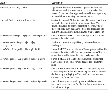
Spark applications consist of transformations and actions. Actions are generally output operations that trigger execution—Spark jobs are only submitted for execution when an output action is performed. Put differently, transformations in Spark are lazy and require an action to fire. In the example, on line 25, saveAsTextFile(..) is an output action that saves the RDD as a text file. Each action results in the execution of a Spark job. Thus each Spark application is a concert between different entities. Table 2-2 explains the difference between them. 6
Table 2-2. Spark Execution Hierarchy
Entity
Description
Application One instance of a SparkContext
Job Set of stages executed as a result of an action
Stage Set of transformations at a shuffle boundary
Task set Set of tasks from the same stage
Task Unit of execution in a stage
Let’s now see how you can build and execute this application. Save the code from Listing 2-1 in a file with a .scala extension, with the following folder structure: ./src/main/scala/FirstApp.scala .
Build
Similar to Java, a Scala application also needs to be compiled into a JAR for deployment and execution. Staying true to pure Scala, this book uses sbt 7 (Simple Build Tool) as the build and dependency manager for all applications. sbt relies on Ivy for dependencies. You can also use the build manager of your choice, including Maven, if you wish.
Create an .sbt file with the following content at the root of the project directory:
name := "FirstApp"
version := "1.0"
scalaVersion := "2.10.5"
sbt by default expects your Scala code to reside in src/main/scala and your test code to reside in src/ test/scala . We recommend creating a fat JAR to house all dependencies using the sbt-assembly plugin. 8 To set up sbt-assembly, create a file at ./project/assembly.sbt and add addSbtPlugin("com.eed3si9n" % "sbt-assembly" % "0.11.2") to it. Creating a fat JAR typically leads to conflicts between binaries and configuration files that share the same relative path. To negate this behavior, sbt-assembly enables you to specify a merge strategy to resolve such conflicts. A reasonable approach is to use the first entry in case of a duplicate, which is what you do here. Add the following to the start of your build definition ( .sbt ) file:
import AssemblyKeys._ assemblySettings
mergeStrategy in assembly <<= (mergeStrategy in assembly) { mergeStrategy => { case entry => {
val strategy = mergeStrategy(entry)
if (strategy == MergeStrategy.deduplicate) MergeStrategy.first else strategy
} }}
To build the application, execute sbt assembly at the command line, with your working directory being the directory where the .sbt file is located. This generates a JAR at ./target/scala-2.10/FirstApp-assembly-1.0.jar .
Execution
Executing a Spark application is very similar to executing a standard Scala or Java program. Spark supports a number of execution modes.
Local Execution
In this mode, the entire application is executed in a single process with potentially multiple threads of execution. Use the following command to execute the application in local mode
$SPARK_HOME/bin/spark-submit --class org.apress.prospark.TranslateApp --master local[n] ./target/scala-2.10/FirstApp-assembly-1.0.jar <app_name> <book_path> <output_path> <language>
where n is the number of threads and should be greater than zero.
Standalone Cluster
In standalone cluster mode , the driver program can be executed on the submission machine (as shown in Figure 2-2 ):
$SPARK_HOME/bin/spark-submit --class org.apress.prospark.TranslateApp --master <master_ url> ./target/scala-2.10/FirstApp-assembly-1.0.jar <app_name> <book_path> <output_path> <language>
Alternatively, the driver can be executed on the cluster (see Figure 2-3 ):
$SPARK_HOME/bin/spark-submit –class org.apress.prospark.TranslateApp --master <master_url> --deploy-mode cluster ./target/scala-2.10/FirstApp-assembly-1.0.jar <app_name> <book_path> <output_path> <language>
Figure 2-2. Standalone cluster deployment with the driver running on the client machine
YARN
Similar to standalone cluster mode, under YARN , 9 the driver program can be executed either on the client
$SPARK_HOME/bin/spark-submit --class org.apress.prospark.TranslateApp --master yarn-client ./target/scala-2.10/FirstApp-assembly-1.0.jar <app_name> <book_path> <output_path> <language>
or on the YARN cluster:
$SPARK_HOME/bin/spark-submit --class org.apress.prospark.TranslateApp --master yarn-cluster ./target/scala-2.10/FirstApp-assembly-1.0.jar <app_name> <book_path> <output_path> <language>
Similar to the distributed cluster mode, the jobs execute on the YARN NodeManager nodes in both cases, and only the execution location of the driver program varies.
The rest of the chapter walks through some of the artifacts introduced in the example application to take a deep dive into the inner workings of Spark.
SparkContext
As mentioned before, SparkContext is the main application entry point. It serves many purposes, some of which are described in this section.
Creation of RDDs
SparkContext has utility functions to create RDDs for many data sources out of the box. Table 2-3 lists some of the common ones. Note that these functions also accept an argument specifying an optional number of slices/number of partitions.
Table 2-3. RDD Creation Methods Exposed by SparkContext
Signature
Description
parallelize[T](seq: Seq[T]): RDD[T] Converts a Scala collection into an RDD.
textFile(path: String): RDD[String] Returns an RDD for a Hadoop text file located at path . Under the hood, it invokes hadoopFile() by using TextInputFormat as the inputFormatClass , LongWriteable as the keyClass , and Text as the
valueClass . It is important to highlight that the key in this case is the position in the file, whereas the value is a line.
9 Spark uses HADOOP_CONF_DIR and YARN_CONF_DIR to access HDFS and talk to the YARN resource manager.
Note that each function returns an RDD with an associated object type. For instance, parallelize() returns a ParallelCollectionRDD (which knows how to serialize and slice up a Scala collection), and textFile() returns a HadoopRDD (which knows how to read data from HDFS and to create partitions). More on RDDs later.
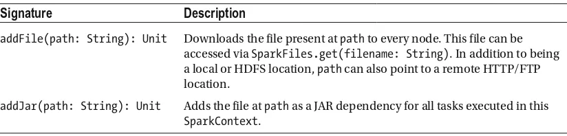
Handling Dependencies
Due to its distributed nature, Spark tasks are parallelized across many worker nodes. Typically, the data (RDDs) and the code (such as closures) are shipped out by Spark; but in certain cases, the task code may require access to an external file or a Java library. The SparkContext instance can also be used to handle these external dependencies (see Table 2-4 ).
SequenceFileInputFormat as the inputFormatClass . API introduced in version 0.21. 10
wholeTextFiles(path: String): RDD[(String, String)]
Returns an RDD for whole Hadoop files located at path . Under the hood, uses String as both the key and the value and WholeTextFileInputFormat as the InputFormatClass . Note that the key is the file path, whereas the value is the entire content of the file(s). Use this method if the files are small. For larger files, use textFile() .
union[T](rdds: Seq[RDD[T]]): RDD[T] Returns an RDD that is the union of all input RDDs of the same type. accessed via SparkFiles.get(filename: String) . In addition to being a local or HDFS location, path can also point to a remote HTTP/FTP location.
Creating Shared Variables
Spark transformations manipulate independent copies of data on worker machines, and thus there is no shared state between them. In certain cases, though, some state may need to be shared across workers and the driver—for instance, if you need to calculate a global value. SparkContext provides two types of shared variables:
• Broadcast variables: As the name suggests, broadcast variables are read-only copies of data broadcast by the driver program to worker tasks—for instance, to share a copy of large variables. Spark by default ships out the data required by each task in a stage. This data is serialized and deserialized before the execution of each task. On the other hand, the data in a broadcast variable is transported via efficient P2P communication and is cached in deserialized form. Therefore, broadcast variables are useful only when they are required across multiple stages in a job. Table 2-5 outlines the creation and use of broadcast variables.
Table 2-5. Broadcast Variable Creation and Use
Signature
Description
broadcast(v: T): Broadcast[T] Broadcasts v to all nodes, and returns a broadcast variable reference. In tasks, the value of this variable can be accessed through the value attribute of the reference object. After creating a broadcast variable, do not use the original variable v in the workers.
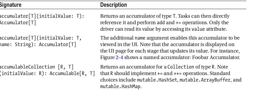
• Accumulators: Accumulators are variables that support associative functions such
as increment . Their prime property is that tasks running on workers can only write to them, and only the driver program can read their value. Thus they are handy for implementing counters or manipulating objects that allow += and/or add operations. Table 2-6 showcases out of the box Accumulators in Spark.
driver can read its value by accessing its value attribute.
accumulator[T](initialValue: T, name: String): Accumulator[T]
The additional name argument enables this accumulator to be viewed in the UI. Note that the accumulator is displayed on the UI page for each stage that updates its value. For instance, Figure 2-4 shows a named accumulator: Foobar Accumulator.
accumulableCollection [R, T]
(initialValue: R): Accumulable[R, T]
Job execution
Transparent to you, SparkContext is also in charge of submitting jobs to the scheduler. These jobs are submitted every time an RDD action is invoked. A job is broken down into stages, which are then broken down into tasks. These tasks are subsequently distributed across the various workers. You will learn more about scheduling in Chapter 4 .
RDD
Resilient distributed datasets (RDDs) lie at the very core of Spark. Almost all data in a Spark application resides in them. Figure 2-5 gives a high-level view of a typical Spark workflow that revolves around the concept of RDDs. As the figure shows, data from an external source or multiple sources is first ingested and converted into an RDD that is then transformed into potentially a series of other RDDs before being written to an external sink or multiple sinks.
Figure 2-5. RDDs in a nutshell
Figure 2-4. Spark UI screenshot of a named accumulator
An RDD in essence is an envelope around data partitions. The persistence level of each RDD is configurable; the default behavior is regeneration under failure. Keeping lineage information—parent RDDs that it depends on—enables RDD regeneration. An RDD is a first-class citizen in the Spark order of things: applications make progress by transforming or actioning RDDs. The base RDD class exposes simple transformations ( map , filter , and so on). Derived classes build on this by extending and implementing three key methods : compute() , getPartitions() , and getDependencies() . For instance, UnionRDD , which takes the union of multiple RDDs, simply returns the partitions and dependencies of the unionized RDDs in its rdd.partitions (public version of getPartitions() ) and rdd.dependencies (sugared version of getDependencies()) methods, respectively. In addition, its compute() method invokes the respective compute() methods of its constituent RDDs.
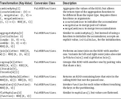
As mentioned, RDDs can also be transformed via implicit conversions. Table 2-8 lists some of these conversion classes.
Table 2-7. Examples of Specialized RDDs
RDD Type
Description
CartesianRDD Obtained as a result of calculating the Cartesian product of two RDDs
HadoopRDD Represents data stored in any Hadoop-compatible store: local FS, HDFS, S3, and HBase
JdbcRDD Contains results of a SQL query execution via a JDBC connection
NewHadoopRDD Same as HadoopRDD but uses the new Hadoop API
ParallelCollectionRDD Contains a Scala Collections object
PipedRDD Used to pipe the contents of an RDD to an external command, such as a
bash command or a Python script
UnionRDD Wrapper around multiple RDDs to treat them as a single RDD
Table 2-8. RDD Conversion Functions
RDD Conversion Class
Description
DoubleRDDFunctions Functions that can be applied to RDDs of Double s. These functions include mean() , variance() , stdev() , and histogram() .
OrderedRDDFunctions Ordering functions that apply to key-value pair RDDs. Functions include sortByKey() .
PairRDDFunctions Functions applicable to key-value pair RDDs. Functions include combineByKey() , aggregateByKey() , reduceByKey() , and groupByKey() .
SequenceFileRDDFunctions Functions to convert key-value pair RDDs to Hadoop SequenceFiles . For example, saveAsSequenceFile() .
Persistence
The persistence level of RDDs explores different points in the space between CPU, IO, and memory cost. This value can be set by making a call to the persist() method exposed by each RDD. The cache() method defaults to a persistence level of MEMORY_ONLY. Persistence is handled by BlockManager , which internally maintains a memory store and a disk store. In addition, RDDs can also be checkpointed using the checkpoint() function. Unlike caching, checkpointing directly saves the RDD to HDFS and does not keep its lineage information.