Pengaruh Faktor Internal dan Faktor Eksternal Terhadap Pemilihan Jalur Konsentrasi Mahasiswa Akuntansi Universitas Katolik Soegijapranata Semarang - Unika Repository

(1)

LAMPIRAN A

Kuesioner

(2)

KUESIONER

Data Responden :

Nama

:

NIM

:

Angkatan

:

Jenis kelamin

: ( ) laki-laki

( ) perempuan

Jalur konsentrasi : ( ) akuntansi keuangan

( ) akuntansi manajemen

( ) sistem informasi

Berikut ini adalah beberapa pertanyaan terkait dengan faktor-faktor apa

yang menjadi pertimbangan anda dalam memilih jalur konsentrasi. Hasil

kuesioner ini diharapkan dapat memberikan masukan bagi jurusan akuntansi

Universitas Katolik Soegijapranata dalam upaya pengembangan jalur konsentrasi

sesuai dengan faktor-faktor yang mempengaruhi mahasiswa dalam pemilihan jalur

konsentrasi tersebut.

(3)

Petunjuk pengisian :

Berikan tanda (

√

) pada jawaban yang anda anggap sesuai dengan penilaian anda

untuk pertanyaan atribut berikut.

1

: sangat tidak setuju

2

:

tidak setuju

3

:

ragu-ragu

4

:

setuju

5

:

sangat setuju

Berikut ini adalah faktor-faktor yang menjadi pertimbangan anda dalam memilih

jalur konsentrasi sesuai dengan pengalaman anda :

No

Pertimbangan saya

1

2

3

4

5

Motivasi diri sendiri jalur AK

1

Ingin

mendapat

pengetahuan

tentang

dimensi-dimensi internasional akuntansi,

pola pengembangan akuntansi internasional

, perbandingan sistem dan praktek akuntansi

di berbagai negara, termasuk issue teknikal

akuntansi internasional dan usaha-usaha

yang telah dilakukan untuk mengurangi

diversitas prinsip dan praktek akuntansi di

negara-negara dunia.

1

2

3

4

5

2

Dapat

membahas,

mendiskusikan dan

menelaah artikel-artikel aktual akuntansi

sebagai penerapan kerangka teoritis dari

teori akuntansi.

1

2

3

4

5

3

Ingin mendapat pengetahuan tentang pasar

modal, mekanisme dan lembaga-lembaga

yang

ada

didalamnya,

mekanisme

perdagangan bursa efek, settlement dan

jenis-jenis sekuritas yang dipedagangkan

serta teori portofolionya.

1

2

3

4

5

4

Ingin

mendapat

pengetahuan

tentang

prosedur, metode dan tehnik analisis

laporan keuangan dan interpretasi terhadap

hasil analisis tersebut.

1

2

3

4

5

(4)

5

Adanya keahlian yang ingin dikembangkan

melalui jalur konsentrasi ini

1

2

3

4

5

Motivasi diri sendiri jalur AM

6

Ingin

membahas,

mendiskusikan

dan

menelaah artikel-artikel dan issue-issue

aktual

akuntansi

dan

perkembangan

akuntansi manajemen sebagai penerapan

kerangka

teoritis

dari

Akuntansi

Manajemen.

1

2

3

4

5

7

Ingin membahas pemeriksaan terhadap

semua

fungsi

manajemen,

yaitu

perencanaan,

pengorganisasian,

pengarahan dan pengawasan untuk menilai

efektivitas, efisiensi dan ekonomisasi dari

setiap fungsi manajemen tersebut sebagai

dasar perbaikan di masa mendatang.

1

2

3

4

5

8

Ingin

mendapat

pengetahuan

tentang

internal auditing, proses pemeriksaan yang

dilakukan internal auditor dan berbagai

peraturan

yang

berkaitan

dengan

pemeriksaan internal, dan kedudukan serta

peran internal audito tentang

temuan-temuan

audit,

pelaporannya

serta

tanggapan atas laporan audit.

1

2

3

4

5

9

Ingin

mendapat

pemahaman

tentang

penyusunan perencanaan dan pengendalian

laba komprehensif, baik laba taktis jangka

pendek maupun laba strategis jangka

panjang.

1

2

3

4

5

10

melalui jalur konsentrasi ini

1

2

3

4

5

Motivasi diri sendiri jalur SIA

11

Ingin mempelajari berbagai aplikasi TI

dalam bisnis yang ada dewasa ini dan

perubahan manajemen sistem informasi

dalam organisasi. Mata kuliah ini juga akan

membahas lebih lanjut tentang tantangan

manajemen dalam era informasi.

1

2

3

4

5

12

Ingin mendapat pemahaman konsep dan

aplikasi sistem manajemen basis data yang

memungkinkan mahasiswa memahami dan

mampu mendesain serta membangun

struktur basis data yang efektif dan efisien.

1

2

3

4

5

(5)

13

Ingin mendapat pengetahuan mahasiswa

konsep dan aplikasi pengembangan sistem

informasi berbasis komputer. Pembahasan

mencakup antara lain konsep, tools, teknik

dan aplikasi-aplikasinya. Secara umum,

mata kuliah ini memberikan tekanan pada

tahap analisis dan perancangan. Meskipun

demikian

untuk

melengkapi

siklus

pengembangan system, mata kuiah ini juga

akan memberikan bahasan secara ringkas

tentang

tahap-tahap

konstruksi

dan

implementasi, serta operasi dan dukungan

system.

1

2

3

4

5

14

Ingin

mendapat

pengetahuan

dan

ketrampilan teknis pemrograman aplikasi

berbasis data yang merupakan tipe dari

aplikasi-aplikasi

sistem

informasi

akuntansi dan manajemen. Ketrampilan ini

akan

memperkuat

kemampuan

untuk

mempersiapkan mahasiswa menjasi analis

sistem dan auditor sistem informasi.

1

2

3

4

5

15

melalui jalur konsentrasi ini

1

2

3

4

5

Motivasi Orang lain

16

Saran dari teman / yang sudah memilih jalur

konsentrasi tersebut

1

2

3

4

5

17

Saran dari orang tua

1

2

3

4

5

18

Banyak peminat/ banyak teman pada bidang

konsentrasi tersebut

1

2

3

4

5

Content

kuliah

19

Dosen yang mengajar menarik

1

2

3

4

5

20

Dosen yang mengajar menguasai materi

kuliah yang disampaikan

1

2

3

4

5

21

Materi kuliah disajikan secara menarik

1

2

3

4

5

22

Distribusi penilaian yang diberikan

1

2

3

4

5

Keterkaitan mata kuliah jalur AK

23

Saya menguasai mata kuliah Teori

Akuntansi (TA)

1

2

3

4

5

24

Saya menguasai mata kuliah Manajemen

Keuangan (MK)

1

2

3

4

5

25

Saya menguasai mata kuliah AKM II

1

2

3

4

5

26

Saya menguasai mata kuliah Statistik

1

2

3

4

5

(6)

27

Saya menguasai mata kuliah Akuntansi

Manajemen (Akmen)

1

2

3

4

5

Keterkaitan mata kuliah jalur AM

28

Saya menguasai mata kuliah Manajemen

Keuangan (MK)

1

2

3

4

5

29

Saya menguasai mata kuliah Akuntansi

Manajemen (Akmen)

1

2

3

4

5

30

Saya menguasai mata kuliah Pemeriksaan

Akuntansi

1

2

3

4

5

Keterkaitan mata kuliah jalur SIA

31

Saya menguasai mata kuliah pengantar

Aplikom lanjutan

1

2

3

4

5

32

Saya menguasai mata kuliah Sistem

Informasi Akuntansi (SIA)

1

2

3

4

5

Faktor eksternal

33

Rencana studi yang akan saya ambil setelah

lulus jenjang s1 mempengaruhi bidang

konsentrasi

1

2

3

4

5

34

Lapangan kerja setelah lulus

1

2

3

4

5

Relevansi

pengkonsentrasian

di

jurusan akuntansi

35

Pengkonsentrasian di jurusan akuntansi

sebaiknya tetap dilakukan

1

2

3

4

5

Nilai terakhir mata kuliah berikut :

A

AB

B

BC

C

CD

D

E

Teori Akuntansi (TA)

Manajemen Keuangan (MK)

AKM II

Statistik

Akuntansi Manajemen (Akmen)

Pemeriksaan Akuntansi

Pengantar aplikom lanjutan

Sistem Informasi Akuntansi (SIA)

(7)

LAMPIRAN B

Statistic descriptive

(8)

1. Statistic descriptive jalur akuntansi keuangan

Mahasiswa perempuan angkatan 2002

Descriptive Statistics

N Minimum Maximum Mean Std. Deviation Motivasi Diri AK 3 16.00 18.00 16.6667 1.15470 Motivasi Org Lain ₃ _9.00 _12.00 _11.0000 _1.73205 Conten Kuliah 3 13.00 15.00 14.3333 1.15470 keterkaitan MK AK 3 18.00 22.00 20.0000 2.00000 Faktor Eksternal ₃ _6.00 _9.00 _7.3333 _1.52753

Valid N (listwise) 3

Mahasiswa laki-laki angkatan 2002

Descriptive Statistics

N Minimum Maximum Mean Std. Deviation Motivasi Diri AK 4 13.00 20.00 16.2500 2.98608 Motivasi Org Lain 4 5.00 11.00 7.5000 2.64575 Conten Kuliah ₄ _7.00 _18.00 _12.0000 _4.54606 keterkaitan MK AK 4 14.00 24.00 18.5000 4.12311 Faktor Eksternal 4 8.00 8.00 8.0000 .00000

Mahasiswa perempuan angkatan 2003

Descriptive Statistics

N Minimum Maximum Mean Std. Deviation Motivasi Diri AK ₄₃ _8.00 _20.00 _15.6512 _2.25604 Motivasi Org Lain 43 3.00 15.00 8.9070 3.09234 Conten Kuliah 43 6.00 19.00 13.4186 3.00185 keterkaitan MK AK ₄₃ _10.00 _25.00 _17.0930 _2.52430 Faktor Eksternal ₄₃ _4.00 _10.00 _7.6977 _1.38933

(9)

Mahasiswa laki-laki angkatan 2003

Descriptive Statistics

N Minimum Maximum Mean Std. Deviation Motivasi Diri AK ₁₁ _5.00 _16.00 _12.4545 _3.88236 Motivasi Org Lain 11 6.00 13.00 8.8182 2.40076 Conten Kuliah 11 8.00 17.00 12.9091 2.46798 keterkaitan MK AK ₁₁ _10.00 _20.00 _16.0909 _2.77325 Faktor Eksternal ₁₁ _6.00 _10.00 _7.8182 _.98165

2. Statistic descriptive jalur akuntansi manajemen

Mahasiswa laki-laki angkatan 2002

Descriptive Statistics

N Minimum Maximum Mean Std. Deviation Motivasi Diri AM 10 11.00 19.00 16.1000 2.18327 Motivasi Org Lain 10 6.00 13.00 8.9000 3.14289 Conten Kuliah ₁₀ _9.00 _20.00 _14.6000 _3.06232 keterkaitan MK AM 10 8.00 15.00 10.5000 2.22361 Faktor Eksternal 10 4.00 10.00 7.2000 1.93218

Mahasiswa perempuan angkatan 2003

Descriptive Statistics

N Minimum Maximum Mean Std. Deviation Motivasi Diri AM 42 12.00 19.00 16.0476 1.49719 Motivasi Org Lain 42 3.00 14.00 9.3810 2.83663 Conten Kuliah 42 9.00 20.00 14.4286 2.81237 keterkaitan MK AM ₄₂ _7.00 _12.00 _9.9048 _1.46187 Faktor Eksternal 42 2.00 10.00 7.2143 1.93221

(10)

Mahasiswa laki-laki angkatan 2003

Descriptive Statistics

N Minimum Maximum Mean Std. Deviation Motivasi Diri AM ₁₆ _14.00 _19.00 _15.6875 _1.35247 Motivasi Org Lain 16 6.00 12.00 9.2500 1.91485 Conten Kuliah 16 5.00 20.00 14.2500 3.54965 keterkaitan MK AM ₁₆ _6.00 _12.00 _9.7500 _1.43759 Faktor Eksternal ₁₆ _5.00 _10.00 _7.3750 _1.31022

3.

Statistic descriptive jalur sistem informasi

Mahasiswa perempuan angkatan 2002

Descriptive Statistics

N Minimum Maximum Mean Std. Deviation Motivasi diri sia ₃ _16.00 _20.00 _18.6667 _2.30940 Motivasi Org Lain 3 5.00 11.00 7.3333 3.21455 Conten Kuliah 3 14.00 17.00 15.6667 1.52753 Keterkaitan MK SIA 3 6.00 8.00 7.0000 1.00000 Faktor Eksternal ₃ _6.00 _7.00 _6.6667 _.57735

Valid N (listwise) ₃

Mahasiswa laki-laki angkatan 2002

Descriptive Statistics

N Minimum Maximum Mean Std. Deviation Motivasi diri sia 4 18.00 20.00 19.5000 1.00000 Motivasi Org Lain 4 3.00 13.00 7.5000 4.43471 Conten Kuliah ₄ _18.00 _20.00 _19.2500 _.95743 Keterkaitan MK SIA 4 8.00 10.00 9.0000 1.15470 Faktor Eksternal 4 6.00 10.00 9.0000 2.00000

Valid N (listwise) ₄

(11)

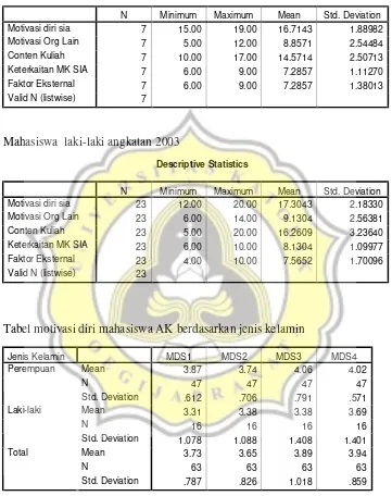
Mahasiswa perempuan angkatan 2003

Descriptive Statistics

N Minimum Maximum Mean Std. Deviation Motivasi diri sia 7 15.00 19.00 16.7143 1.88982 Motivasi Org Lain 7 5.00 12.00 8.8571 2.54484 Conten Kuliah 7 10.00 17.00 14.5714 2.50713 Keterkaitan MK SIA ₇ _6.00 _9.00 _7.2857 _1.11270 Faktor Eksternal 7 6.00 9.00 7.2857 1.38013

Mahasiswa laki-laki angkatan 2003

Descriptive Statistics

N Minimum Maximum Mean Std. Deviation Motivasi diri sia 23 12.00 20.00 17.3043 2.18330 Motivasi Org Lain ₂₃ _6.00 _14.00 _9.1304 _2.56381 Conten Kuliah 23 5.00 20.00 16.2609 3.23640 Keterkaitan MK SIA 23 6.00 10.00 8.1304 1.09977 Faktor Eksternal ₂₃ _4.00 _10.00 _7.5652 _1.70096

Valid N (listwise) ₂₃

Tabel motivasi diri mahasiswa AK berdasarkan jenis kelamin

Jenis Kelamin MDS1 MDS2 MDS3 MDS4 Mean _3.87 _3.74 _4.06 _4.02

N 47 47 47 47

Perempuan

Std. Deviation _.612 _.706 _.791 _.571 Mean _3.31 _3.38 _3.38 _3.69

N 16 16 16 16

Laki-laki

Std. Deviation 1.078 1.088 1.408 1.401 Mean _3.73 _3.65 _3.89 _3.94

N ₆₃ ₆₃ ₆₃ ₆₃

Total

Std. Deviation .787 .826 1.018 .859

(12)

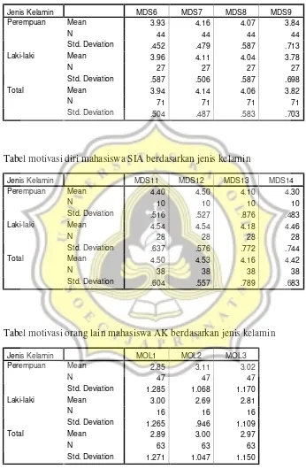
Tabel motivasi diri mahasiswa AM berdasarkan jenis kelamin

Jenis Kelamin MDS6 MDS7 MDS8 MDS9 Mean _3.93 _4.16 _4.07 _3.84

N 44 44 44 44

Perempuan

Std. Deviation .452 .479 .587 .713 Mean _3.96 _4.11 _4.04 _3.78

N 27 27 27 27

Laki-laki

Std. Deviation _.587 _.506 _.587 _.698 Mean 3.94 4.14 4.06 3.82

N 71 71 71 71

Total

Std. Deviation _.504 _.487 _.583 _.703

Tabel motivasi diri mahasiswa SIA berdasarkan jenis kelamin

Jenis Kelamin MDS11 MDS12 MDS13 MDS14 Mean 4.40 4.50 4.10 4.30

N 10 10 10 10

Perempuan

N 28 28 28 28

Laki-laki

N ₃₈ ₃₈ ₃₈ ₃₈

Total

Std. Deviation .604 .557 .789 .683

Tabel motivasi orang lain mahasiswa AK berdasarkan jenis kelamin

Jenis Kelamin MOL1 MOL2 MOL3 Mean 2.85 3.11 3.02

N 47 47 47

Perempuan

Std. Deviation _1.285 _1.068 _1.170 Mean 3.00 2.69 2.81

N 16 16 16

Laki-laki

Std. Deviation _1.265 _.946 _1.109 Mean 2.89 3.00 2.97

N ₆₃ ₆₃ ₆₃

Total

Std. Deviation 1.271 1.047 1.150

(13)

Tabel motivasi orang lain mahasiswa AM berdasarkan jenis kelamin

N 44 44 44

Perempuan

Std. Deviation _1.128 _1.169 _1.160 Mean 3.30 2.56 3.11

N 27 27 27

Laki-laki

Std. Deviation 1.068 .974 1.121 Mean _3.28 _2.87 _3.07

N 71 71 71

Total

Std. Deviation 1.098 1.120 1.138

Tabel motivasi orang lain mahasiswa SIA berdasarkan jenis kelamin

N 10 10 10

Perempuan

Std. Deviation 1.101 1.229 1.337 Mean _3.36 _2.82 _2.89

N 28 28 28

Laki-laki

Std. Deviation 1.129 1.249 1.257 Mean _3.24 _2.66 _3.00

N ₃₈ ₃₈ ₃₈

Total

Std. Deviation 1.125 1.258 1.273

(14)

LAMPIRAN C

Validitas

(15)

1.

faktor analisis jalur akuntansi keuangan

Factor Analysis

KMO and Bartlett's Test

Kaiser-Meyer-Olkin Measure of Sampling

Adequacy. _.827

Approx. Chi-Square 1227.496

df ₁₇₁

Bartlett's Test of Sphericity

Sig. .000

Communalities

Initial Extraction MDS1 _1.000 _.686 MDS2 1.000 .676 MDS3 _1.000 _.718 MDS4 _1.000 _.747 MDS5 1.000 .398 MOL1 1.000 .689 MOL2 1.000 .625 MOL3 _1.000 _.630 CK1 1.000 .621 CK2 1.000 .696 CK3 _1.000 _.727 CK4 1.000 .670 KMK1 1.000 .603 KMK2 1.000 .664 KMK3 1.000 .673 KMK4 _1.000 _.612 KMK5 1.000 .566 FE1 1.000 .713 FE2 1.000 .683

Extraction Method: Principal Component Analysis.

(16)

Total Variance Explained

Comp

onent Initial Eigenvalues

Extraction Sums of Squared Loadings

Rotation Sums of Squared Loadings

Total

% of Variance

Cumulative

% Total

% of Variance

Cumulative

% Total

% of Variance

Cumulative % 1 5.072 26.692 26.692 5.072 26.692 26.692 2.994 15.758 15.758 2 2.731 14.376 41.068 2.731 14.376 41.068 2.945 15.500 31.258 3 _2.034 _10.707 _51.775 _2.034 _10.707 _51.775 _2.868 _15.092 _46.350 4 1.350 7.108 58.883 1.350 7.108 58.883 2.020 10.631 56.982 5 1.209 6.363 65.246 1.209 6.363 65.246 1.570 8.264 65.246

6 .798 4.202 69.448

7 _.676 _3.556 _73.004

8 .642 3.378 76.382

9 .621 3.270 79.652

10 _.537 _2.827 _82.479

11 _.501 _2.635 _85.114

12 .470 2.474 87.589

13 .423 2.224 89.813

14 _.386 _2.032 _91.844

15 _.365 _1.919 _93.764

16 .343 1.806 95.570

17 .310 1.634 97.204

18 .282 1.487 98.690

19 _.249 _1.310 _100.000

Component Matrix(a)

Component

1 2 3 4 5

MDS1 .544 -.406

MDS2 _.561 _-.490

MDS3 .537 -.484

MDS4 .552 -.468 .415

MDS5 .438

MOL1 _.464 _.441

MOL2 -.410

MOL3 _.546

CK1 .405 .656

CK2 .585 .507

CK3 _.502 _.594

CK4 .515 .591

KMK1 .525 -.432

KMK2 _.572 _-.557

KMK3 .571

KMK4 _.594 _-.413

KMK5 .616

FE1 .410 .528 .506

FE2 _.613

Extraction Method: Principal Component Analysis. a 5 components extracted.

(17)

Rotated Component Matrix(a)

Component

1 2 3 4 5

MDS1 .810

MDS2 .774

MDS3 _.830

MDS4 _.844

MDS5 _.550

MOL1 .785

MOL2 _.775

MOL3 _.722

CK1 .704

CK2 .781

CK3 _.839

CK4 _.787

KMK1 .742

KMK2 .778

KMK3 _.788

KMK4 .725

KMK5 .666

FE1 .816

FE2 _.787

Extraction Method: Principal Component Analysis. Rotation Method: Varimax with Kaiser Normalization. a Rotation converged in 6 iterations.

Component Transformation Matrix

Component 1 2 3 4 5

1 .572 .487 .489 .356 .263

2 _-.270 _.731 _-.570 _.255 _-.051 3 _-.689 _-.011 _.534 _.476 _-.118 4 _-.353 _.217 _.157 _-.496 _.747 5 .030 -.426 -.354 .579 .597

Extraction Method: Principal Component Analysis. Rotation Method: Varimax with Kaiser Normalization.

(18)

2

.

faktor analisis jalur akuntansi manajemen

Factor Analysis

KMO and Bartlett's Test

Adequacy. _.797

df ₁₃₆

Sig. .000

Communalities

Initial Extraction MDS6 _1.000 _.630 MDS7 1.000 .704 MDS8 _1.000 _.675 MDS9 _1.000 _.614 MDS10 1.000 .438 MOL1 1.000 .706 MOL2 1.000 .645 MOL3 _1.000 _.637 CK1 1.000 .599 CK2 1.000 .688 CK3 _1.000 _.730 CK4 1.000 .679 KMK2 1.000 .678 KMK5 1.000 .655 KMK6 1.000 .652 FE1 _1.000 _.700 FE2 1.000 .709

(19)

Comp

Total

% of Variance

Cumulative

% Total

% of Variance

Cumulative

% Total

% of Variance

Cumulativ e % 1 4.756 27.979 27.979 4.756 27.979 27.979 2.941 17.299 17.299 2 2.129 12.522 40.501 2.129 12.522 40.501 2.634 15.496 32.794 3 _1.821 _10.715 _51.215 _1.821 _10.715 _51.215 _2.032 _11.955 _44.750 4 1.334 7.848 59.063 1.334 7.848 59.063 1.983 11.667 56.417 5 1.100 6.471 65.535 1.100 6.471 65.535 1.550 9.118 65.535

6 .837 4.925 70.460

7 _.697 _4.099 _74.559

8 .625 3.674 78.233

9 .604 3.553 81.786

10 _.528 _3.105 _84.892

11 _.489 _2.874 _87.765

12 .457 2.688 90.453

13 .365 2.148 92.602

14 _.355 _2.086 _94.688

15 _.337 _1.984 _96.672

16 .302 1.778 98.450

17 .264 1.550 100.000

Component Matrix(a)

Component

₁ ₂ ₃ ₄ ₅

MDS6 _.439 _.610

MDS7 .548 .571

MDS8 .545 .593

MDS9 _.475 _.591

MDS10 .476

MOL1 .545 -.411 .462

MOL2 .531

MOL3 _.600

CK1 .612

CK2 _.656 _-.410

CK3 .671

CK4 .655

KMK2 _.410 _.531

KMK5 .539 .509

KMK6 .571 .406

FE1 _.454

FE2 .510 .507

(20)

Component

1 2 3 4 5

MDS6 .784

MDS7 _.804

MDS8 .781

MDS9 .746

MDS10 .521

MOL1 _.773

MOL2 .798

MOL3 .716

CK1 _.706

CK2 .767

CK3 _.822

CK4 .795

KMK2 .804

KMK5 _.737

KMK6 .736

FE1 .793

FE2 .812

Component Transformation Matrix

Component 1 2 3 4 5

1 .631 .471 .402 .400 .244

2 _-.493 _.825 _-.210 _.105 _-.144 3 _-.360 _.092 _.641 _-.475 _.475 4 -.434 -.272 -.001 .728 .455 5 .205 .121 -.619 -.270 .698

(21)

3

.

faktor analisis jalur system informasi

Factor Analysis

KMO and Bartlett's Test

Adequacy. _.820

df ₁₂₀

Sig. .000

Communalities

Initial Extraction MDS11 _1.000 _.769 MDS12 1.000 .801 MDS13 _1.000 _.794 MDS14 _1.000 _.807 MDS15 1.000 .392 MOL1 1.000 .662 MOL2 1.000 .633 MOL3 _1.000 _.640 CK1 1.000 .588 CK2 1.000 .694 CK3 _1.000 _.736 CK4 1.000 .675 KMK7 1.000 .724 KMK8 1.000 .851 FE1 1.000 .667 FE2 _1.000 _.747

(22)

Comp

Total

% of Variance

Cumulative

% Total

% of Variance

Cumulative

% Total

% of Variance

Cumulative % 1 4.827 30.168 30.168 4.827 30.168 30.168 3.219 20.116 20.116 2 2.398 14.988 45.156 2.398 14.988 45.156 2.930 18.311 38.427 3 _1.721 _10.757 _55.913 _1.721 _10.757 _55.913 _2.050 _12.813 _51.240 4 1.346 8.410 64.323 1.346 8.410 64.323 1.582 9.889 61.130 5 .890 5.560 69.883 .890 5.560 69.883 1.401 8.753 69.883

6 .803 5.019 74.902

7 _.622 _3.890 _78.793

8 .587 3.666 82.458

9 .533 3.330 85.789

10 _.465 _2.908 _88.697

11 _.397 _2.483 _91.180

12 .370 2.315 93.495

13 .311 1.945 95.440

14 _.288 _1.797 _97.237

15 _.233 _1.457 _98.695

16 .209 1.305 100.000

Component Matrix(a)

Component

₁ ₂ ₃ ₄ ₅

MDS11 .624 -.569

MDS12 .704 -.524

MDS13 .655 -.589

MDS14 .622 -.593

MDS15 _.511

MOL1 .452 .406

MOL2 .505 -.402

MOL3 .465 .434

CK1 _.594

CK2 .617 .409

CK3 _.684

CK4 .719

KMK7 .467 .631

KMK8 _.490 _.688

FE1 .416 .554

FE2 .585 .438

(23)

Component

1 2 3 4 5

MDS11 .858

MDS12 _.865

MDS13 .861

MDS14 .892

MDS15 .517

MOL1 _.778

MOL2 .786

MOL3 .751

CK1 _.685

CK2 .805

CK3 _.822

CK4 .748

KMK7 .704

KMK8 _.882

FE1 .773

FE2 .854

Component Transformation Matrix

Component 1 2 3 4 5

1 _.604 _.637 _.309 _.235 _.280

2 -.740 .429 .513 .072 -.008 3 _-.277 _.090 _-.553 _.607 _.491 4 _.094 _-.585 _.541 _.595 _.034 5 -.051 -.243 .207 -.465 .824

(24)

LAMPIRAN D

Reliabilitas

(25)

Reliability

****** Method 2 (covariance matrix) will be used for this analysis ******

_

R E L I A B I L I T Y A N A L Y S I S - S C A L E (A L P H A)

Mean Std Dev Cases

1. MDS1 3.5988 .9091 172.0

2. MDS2 3.6395 .8841 172.0

3. MDS3 3.6512 1.0233 172.0

4. MDS4 3.7674 .8809 172.0

Correlation Matrix

MDS1 MDS2 MDS3 MDS4

MDS1 1.0000

MDS2 .5976 1.0000

MDS3 .5905 .5583 1.0000

MDS4 .5839 .6426 .6685 1.0000

N of Cases = 172.0

N of

Statistics for Mean Variance Std Dev Variables

Scale 14.6570 9.6419 3.1051 4

Item-total Statistics

Scale Scale Corrected

Mean Variance Item- Squared Alpha

if Item if Item Total Multiple if Item

Deleted Deleted Correlation Correlation Deleted

MDS1 11.0581 5.8212 .6826 .4688 .8288

MDS2 11.0174 5.8886 .6926 .4956 .8251

MDS3 11.0058 5.2807 .7046 .5150 .8228

MDS4 10.8895 5.7246 .7452 .5653 .8043

Reliability Coefficients 4 items

Alpha = .8588 Standardized item alpha = .8606

(26)

Reliability

_

Mean Std Dev Cases

1. MDS6 3.5291 .8613 172.0

2. MDS7 3.6919 .9134 172.0

3. MDS8 3.7849 .8687 172.0

4. MDS9 3.7093 .8358 172.0

Correlation Matrix

MDS6 MDS7 MDS8 MDS9

MDS6 1.0000

MDS7 .5801 1.0000

MDS8 .4891 .5424 1.0000

MDS9 .4098 .4948 .5819 1.0000

N of Cases = 172.0

N of

Scale 14.7151 7.7254 2.7795 4

Deleted Deleted Correlation Correlation Deleted

MDS6 11.1860 4.7488 .5953 .3830 .7774

MDS7 11.0233 4.3620 .6628 .4498 .7452

MDS8 10.9302 4.5331 .6590 .4480 .7473

MDS9 11.0058 4.8362 .5959 .3874 .7771

(27)

Reliability

_

Mean Std Dev Cases

1. MDS11 3.7849 .9764 172.0

2. MDS12 3.7384 .9279 172.0

3. MDS13 3.6221 .8867 172.0

4. MDS14 3.7674 .9199 172.0

Correlation Matrix

MDS11 MDS12 MDS13 MDS14

MDS11 1.0000

MDS12 .6991 1.0000

MDS13 .6621 .7534 1.0000

MDS14 .7318 .7094 .7233 1.0000

N of Cases = 172.0

N of

Scale 14.9128 10.8052 3.2871 4

MDS11 11.1279 6.1239 .7714 .6065 .8893

MDS12 11.1744 6.2267 .8028 .6543 .8771

MDS13 11.2907 6.4530 .7916 .6447 .8815

MDS14 11.1453 6.2536 .8054 .6523 .8762

(28)

Reliability

_

Mean Std Dev Cases

1. MOL1 3.1279 1.1777 172.0

2. MOL2 2.8721 1.1270 172.0

3. MOL3 3.0174 1.1672 172.0

Correlation Matrix

MOL1 MOL2 MOL3

MOL1 1.0000

MOL2 .4750 1.0000

MOL3 .5216 .4107 1.0000

N of Cases = 172.0

N of

Scale 9.0174 7.7950 2.7920 3

Scale Scale Corrected

MOL1 5.8895 3.7129 .5938 .3539 .5820

MOL2 6.1453 4.1834 .5079 .2621 .6856

MOL3 6.0000 3.9181 .5442 .3064 .6437

(29)

Reliability

_

Mean Std Dev Cases

1. CK1 3.2733 1.1347 172.0

2. CK2 3.8663 .8981 172.0

3. CK3 3.7733 .9495 172.0

4. CK4 3.4477 .9868 172.0

Correlation Matrix

CK1 CK2 CK3 CK4

CK1 1.0000

CK2 .5181 1.0000

CK3 .5192 .5815 1.0000

CK4 .5012 .5958 .6270 1.0000

N of Cases = 172.0

N of

Scale 14.3605 10.4892 3.2387 4

CK1 11.0872 5.9046 .5979 .3593 .8187

CK2 10.4942 6.5789 .6737 .4590 .7789

CK3 10.5872 6.3023 .6892 .4869 .7698

CK4 10.9128 6.1619 .6845 .4891 .7708

(30)

Reliability

Mean Std Dev Cases

1. KMK1 3.0116 .7872 172.0

2. KMK2 3.1453 .8494 172.0

3. KMK3 3.1395 .8117 172.0

4. KMK4 3.0698 .8348 172.0

5. KMK5 3.4419 .8251 172.0

Covariance Matrix

KMK1 KMK2 KMK3 KMK4 KMK5

KMK1 .6197

KMK2 .3550 .7214

KMK3 .3317 .3656 .6588

KMK4 .2740 .3407 .3469 .6969

KMK5 .2638 .3389 .2947 .3725 .6808

Correlation Matrix

KMK1 KMK2 KMK3 KMK4 KMK5

KMK1 1.0000

KMK2 .5309 1.0000

KMK3 .5191 .5303 1.0000

KMK4 .4170 .4805 .5120 1.0000

KMK5 .4062 .4836 .4401 .5408 1.0000

N of Cases = 172.0

if Item if Item Total Multiple if Item

KMK1 12.7965 6.8765 .5932 .3751 .7986

KMK2 12.6628 6.4236 .6504 .4296 .7820

KMK3 12.6686 6.6088 .6417 .4217 .7848

KMK4 12.7384 6.5803 .6230 .4084 .7901

KMK5 12.3663 6.7247 .5935 .3737 .7986

(31)

Reliability

Mean Std Dev Cases

1. KMK2 3.1453 .8494 172.0

2. KMK5 3.4419 .8251 172.0

3. KMK6 3.3547 .7546 172.0

Correlation Matrix

KMK2 KMK5 KMK6

KMK2 1.0000

KMK5 .4836 1.0000

KMK6 .4392 .4982 1.0000

N of Cases = 172.0

N of

Scale 9.9419 3.8329 1.9578 3

KMK2 6.7965 1.8706 .5340 .2861 .6633

KMK5 6.5000 1.8538 .5778 .3351 .6074

KMK6 6.5872 2.0801 .5437 .2995 .6517

(32)

Reliability

_

Mean Std Dev Cases

1. KMK7 3.8895 .7129 172.0

2. KMK8 3.5814 .7249 172.0

Correlation Matrix

KMK7 KMK8

KMK7 1.0000

KMK8 .4758 1.0000

N of Cases = 172.0

N of

Scale 7.4709 1.5255 1.2351 2

Mean Variance Item- Squared Alpha

KMK7 3.5814 .5255 .4758 .2264 .

KMK8 3.8895 .5082 .4758 .2264 .

(33)

Reliability

Mean Std Dev Cases

1. FE1 3.5698 .9182 172.0

2. FE2 3.9419 .9222 172.0

Correlation Matrix

FE1 FE2

FE1 1.0000

FE2 .4537 1.0000

N of Cases = 172.0

N of

Scale 7.5116 2.4619 1.5690 2

FE1 3.9419 .8504 .4537 .2059 .

FE2 3.5698 .8431 .4537 .2059 .

(34)

LAMPIRAN E

Regresi Logistik

(35)

1. Regresi logistik konsentrasi akuntansi keuangan

Logistic Regression

Case Processing Summary

Unweighted Cases(a) N Percent

Included in Analysis ₁₇₂ _100.0

Missing Cases 0 .0

Selected Cases

Total ₁₇₂ _100.0

Unselected Cases 0 .0

Total ₁₇₂ _100.0

a If weight is in effect, see classification table for the total number of cases.

Dependent Variable Encoding

Original Value Internal Value

non ak 0

ak ₁

Block 0: Beginning Block

Iteration History(a,b,c)

Coefficients

Iteration

-2 Log

likelihood Constant

1 _225.996 _-.535

2 _225.989 _-.548

Step 0

3 225.989 -.548

a Constant is included in the model. b Initial -2 Log Likelihood: 225.989

c Estimation terminated at iteration number 3 because parameter estimates changed by less than .001.

Classification Table(a,b)

Observed Predicted

akt keu

non ak ak

Percentage Correct

akt keu non ak ₁₀₉ ₀ _100.0

ak 63 0 .0

Step 0

Overall Percentage _63.4

a Constant is included in the model. b The cut value is .500

Variables in the Equation

B S.E. Wald df Sig. Exp(B)

Step 0 Constant _-.548 _.158 _11.999 ₁ _.001 _.578

(36)

Variables not in the Equation

Score df Sig.

MDSAK _3.130 ₁ _.077

MOL .330 1 .566

CK _11.339 ₁ _.001

KMKAK _18.774 ₁ _.000

Variables

FE 1.417 1 .234

Step 0

Overall Statistics _39.814 ₅ _.000

Block 1: Method = Enter

Iteration History(a,b,c,d)

Coefficients

Iteration

-2 Log

likelihood Constant MDSAK MOL CK KMKAK FE

1 182.915 -1.748 .006 .013 -.220 .248 .032

2 _177.211 _-2.815 _.009 _.035 _-.313 _.384 _.010

3 176.911 -3.121 .011 .040 -.339 .425 -.005

4 _176.909 _-3.142 _.011 _.041 _-.341 _.428 _-.006

Step 1

5 176.909 -3.142 .011 .041 -.341 .428 -.006

a Method: Enter

b Constant is included in the model. c Initial -2 Log Likelihood: 225.989

d Estimation terminated at iteration number 5 because parameter estimates changed by less than .001.

Omnibus Tests of Model Coefficients

Chi-square df Sig.

Step _49.080 ₅ _.000

Block 49.080 5 .000

Step 1

Model _49.080 ₅ _.000

Model Summary

Step

-2 Log likelihood

Cox & Snell R Square

Nagelkerke R Square

1 176.909 .248 .339

Hosmer and Lemeshow Test

Step Chi-square df Sig.

1 3.695 8 .884

(37)

Contingency Table for Hosmer and Lemeshow Test

akt keu = non ak akt keu = ak

Observed Expected Observed Expected Total

1 16 16.412 1 .588 17

2 ₁₇ _15.264 ₀ _1.736 ₁₇

3 14 14.338 3 2.662 17

4 ₁₂ _13.326 ₅ _3.674 ₁₇

5 11 12.251 6 4.749 17

6 ₁₁ _10.665 ₆ _6.335 ₁₇

7 9 9.392 8 7.608 17

8 ₉ _8.096 ₈ _8.904 ₁₇

9 6 5.669 11 11.331 17

Step 1

10 ₄ _3.588 ₁₅ _15.412 ₁₉

Classification Table(a)

Observed Predicted

akt keu

non ak ak

Percentage Correct

akt keu non ak ₉₄ ₁₅ _86.2

ak 29 34 54.0

Step 1

a The cut value is .500

Variables in the Equation

MDSAK _.011 _.072 _.025 ₁ _.875 _1.011

MOL .041 .078 .271 1 .603 1.042

CK _-.341 _.076 _20.337 ₁ _.000 _.711

KMKAK .428 .092 21.439 1 .000 1.534

FE _-.006 _.136 _.002 ₁ _.963 _.994

Step 1(a)

Constan

t -3.142 1.457 4.648 1 .031 .043

a Variable(s) entered on step 1: MDSAK, MOL, CK, KMKAK, FE.

(38)

Correlation Matrix

Constant MDSAK MOL CK KMKAK FE

Constan

t 1.000 -.311 -.107 -.104 -.413 -.284

MDSAK _-.311 _1.000 _-.176 _.034 _-.193 _-.225

MOL -.107 -.176 1.000 -.385 .037 -.022

CK _-.104 _.034 _-.385 _1.000 _-.450 _.018

KMKAK _-.413 _-.193 _.037 _-.450 _1.000 _-.249

Step 1

FE -.284 -.225 -.022 .018 -.249 1.000

Step number: 1

_

Observed Groups and Predicted Probabilities

16





F



R 12



E



Q



n



U



n



E 8



n



N



n a a a



C



n n a aaa a a



Y



n n n a ann a a a a



4



n nna n n n ann n aaa a na a a a





nnnnnnnnn nnnnn nan nnna naanaaa a a a



nnnnnnnnn nnnnn nnan nnnnannannaa ana aaaanaa a a



nnnnnnnnnnnnnnnannnnannnnnnnnnnnnannn naannnnaaa aaa a n a



Predicted



Prob: 0 .25 .5 .75 1

Group: nnnnnnnnnnnnnnnnnnnnnnnnnnnnnnaaaaaaaaaaaaaaaaaaaaaaaaaaaaaa

Predicted Probability is of Membership for ak

The Cut Value is .50

Symbols: n - non ak

a - ak

Each Symbol Represents 1 Case.

(39)

2. Regresi logistik konsentrasi akuntansi manajemen

Logistic Regression

Case Processing Summary

Missing Cases 0 .0

Selected Cases

Total ₁₇₂ _100.0

non am ₀

am 1

Block 0: Beginning Block

Iteration History(a,b,c)

Coefficients

Iteration

-2 Log

likelihood Constant

1 233.184 -.349

2 _233.183 _-.352

Step 0

3 233.183 -.352

Observed Predicted

akt mnj

non am am

Percentage Correct

akt mnj non am ₁₀₁ ₀ _100.0

am 71 0 .0

Step 0

Variables in the Equation

Step 0 Constant -.352 .155 5.179 1 .023 .703

(40)

Score df Sig.

MDSAM 24.309 1 .000

MOL _.674 ₁ _.412

CK .030 1 .863

KMKAM _.029 ₁ _.866

Variables

FE _2.302 ₁ _.129

Step 0

Overall Statistics 30.119 5 .000

Block 1: Method = Enter

Iteration History(a,b,c,d)

Coefficients

Iteration

-2 Log

likelihood Constant MDSAM MOL CK KMKAM FE

1 198.949 -2.462 .300 -.015 -.044 -.013 -.187

2 _193.654 _-3.901 _.459 _.022 _-.097 _-.034 _-.242

3 193.367 -4.476 .508 .031 -.110 -.038 -.249

4 _193.365 _-4.521 _.511 _.032 _-.111 _-.038 _-.249

Step 1

5 193.365 -4.521 .511 .032 -.111 -.038 -.249

a Method: Enter

Chi-square df Sig.

Step _39.818 ₅ _.000

Block 39.818 5 .000

Step 1

Model _39.818 ₅ _.000

Model Summary

Step

-2 Log likelihood

Nagelkerke R Square

1 193.365 .207 .278

1 3.507 8 .899

(41)

akt mnj = non am akt mnj = am

1 17 16.257 0 .743 17

2 ₁₃ _14.271 ₄ _2.729 ₁₇

3 13 13.116 4 3.884 17

4 ₁₂ _11.838 ₅ _5.162 ₁₇

5 12 10.440 5 6.560 17

6 ₁₀ _9.492 ₇ _7.508 ₁₇

7 7 8.528 10 8.472 17

8 ₆ _7.345 ₁₁ _9.655 ₁₇

9 6 5.760 11 11.240 17

Step 1

10 ₅ _3.954 ₁₄ _15.046 ₁₉

Classification Table(a)

Observed Predicted

akt mnj

non am am

Percentage Correct

akt mnj non am 81 20 80.2

am 30 41 57.7

Step 1

Overall Percentage 70.9

Variables in the Equation

MDSAM .511 .105 23.513 1 .000 1.668

MOL _.032 _.072 _.192 ₁ _.661 _1.032

CK -.111 .070 2.548 1 .110 .895

KMKAM _-.038 _.113 _.113 ₁ _.737 _.963

FE -.249 .125 3.943 1 .047 .780

Step 1(a)

Constan

t -4.521 1.684 7.205 1 .007 .011

a Variable(s) entered on step 1: MDSAM, MOL, CK, KMKAM, FE.

Correlation Matrix

Constant MDSAM MOL CK KMKAM FE

Constan

t 1.000 -.653 -.119 -.028 -.206 -.281

MDSAM _-.653 _1.000 _.022 _-.274 _-.162 _-.084

MOL -.119 .022 1.000 -.406 -.009 -.088

CK _-.028 _-.274 _-.406 _1.000 _-.249 _.040

KMKAM _-.206 _-.162 _-.009 _-.249 _1.000 _-.282

Step 1

FE -.281 -.084 -.088 .040 -.282 1.000

(42)

Step number: 1

8



a





a



a a



F



a a



R 6



a n a aa a a



E



a n a aa a a



Q



n a na a n a aan a a a a



U



n a na a n a aan a a a a



E 4



n n nna aan n anan aaa a a aa a a



N



n n nna aan n anan aaa a a aa a a



C



nnnn n nannnn nnn aan nnnnanaaaanaa aa aa a



Y



nnnn n nannnn nnn aan nnnnanaaaanaa aa aa a



2



nnnn n nannnn nnnnnan nnnnnnanaanaa aanaaa aa a a





nnnn n nannnn nnnnnan nnnnnnanaanaa aanaaa aa a a



nnnn nn nnnnnnnnnnnnannnnnnnnnnnnnannannnnnnnnaanaan



nnnn nn nnnnnnnnnnnnannnnnnnnnnnnnannannnnnnnnaanaan



Predicted



Prob: 0 .25 .5 .75 1

Group: nnnnnnnnnnnnnnnnnnnnnnnnnnnnnnaaaaaaaaaaaaaaaaaaaaaaaaaaaaaa

Predicted Probability is of Membership for am

The Cut Value is .50

Symbols: n - non am

a - am

Each Symbol Represents .5 Cases.

(43)

3. Regresi logistik konsentrasi sistem informasi

Logistic Regression

Case Processing Summary

Missing Cases 0 .0

Selected Cases

Total ₁₇₂ _100.0

non si ₀

si 1

Block 0: Beginning Block

Iteration History(a,b,c)

Coefficients

Iteration

-2 Log

likelihood Constant

1 _182.291 _-1.116

2 181.661 -1.255

3 _181.660 _-1.260

Step 0

4 _181.660 _-1.260

Observed Predicted

sistem

non si si

Percentage Correct

sistem non si 134 0 100.0

si ₃₈ ₀ _.0

Step 0

(44)

Variables in the Equation

Step 0 Constant -1.260 .184 47.019 1 .000 .284

Score df Sig.

MDSSIA _32.916 ₁ _.000

MOL .095 1 .758

CK _16.933 ₁ _.000

KMKSIA 8.129 1 .004

Variables

FE _.175 ₁ _.676

Step 0

Overall Statistics 44.151 5 .000

Block 1: Method = Enter

Iteration History(a,b,c,d)

Coefficients

Iteration

-2 Log

likelihood Constant MDSSIA MOL CK KMKSIA FE

1 _143.537 _-4.989 _.187 _-.099 _.132 _.079 _-.067

2 _130.291 _-8.381 _.333 _-.122 _.212 _.104 _-.121

3 128.075 -10.397 .426 -.125 .258 .094 -.152

4 _127.981 _-10.902 _.450 _-.126 _.271 _.089 _-.161

5 _127.981 _-10.927 _.451 _-.126 _.272 _.088 _-.162

Step 1

6 127.981 -10.927 .451 -.126 .272 .088 -.162

a Method: Enter

Chi-square df Sig.

Step 53.680 5 .000

Block 53.680 5 .000

Step 1

Model _53.680 ₅ _.000

Model Summary

Step

-2 Log likelihood

Nagelkerke R Square

1 127.981 .268 .411

(45)

1 3.456 8 .903

sistem = non si sistem = si

1 17 16.911 0 .089 17

2 ₁₇ _16.714 ₀ _.286 ₁₇

3 16 16.390 1 .610 17

4 ₁₆ _15.879 ₁ _1.121 ₁₇

5 ₁₄ _15.121 ₃ _1.879 ₁₇

6 13 14.265 4 2.735 17

7 ₁₄ _13.101 ₃ _3.899 ₁₇

8 13 11.514 4 5.486 17

9 ₁₀ _9.073 ₇ _7.927 ₁₇

Step 1

10 ₄ _5.033 ₁₅ _13.967 ₁₉

Classification Table(a)

Observed Predicted

sistem

non si si

Percentage Correct

sistem non si ₁₂₆ ₈ _94.0

si 22 16 42.1

Step 1

Variables in the Equation

MDSSIA .451 .106 18.003 1 .000 1.569

MOL _-.126 _.086 _2.130 ₁ _.144 _.882

CK _.272 _.104 _6.773 ₁ _.009 _1.312

KMKSIA .088 .216 .168 1 .682 1.093

FE _-.162 _.153 _1.124 ₁ _.289 _.851

Step 1(a)

Constan

t -10.927 2.319 22.198 1 .000 .000

a Variable(s) entered on step 1: MDSSIA, MOL, CK, KMKSIA, FE.

(46)

Correlation Matrix

Constant MDSSIA MOL CK KMKSIA FE

Constan

t 1.000 -.577 -.144 -.286 -.307 -.158

MDSSIA _-.577 _1.000 _.067 _-.068 _-.171 _-.084

MOL -.144 .067 1.000 -.337 -.030 .017

CK _-.286 _-.068 _-.337 _1.000 _-.228 _-.172

KMKSIA _-.307 _-.171 _-.030 _-.228 _1.000 _-.221

Step 1

FE -.158 -.084 .017 -.172 -.221 1.000

Step number: 1

32





n



F



n



R 24



n



E



n



Q



n



U



n



E 16



n



N



ns



C



nn n



Y



nnnn



8



nnnn s s s





nnnnnnnss ns n s



nnnnnnnnnnnn nn nnn s n s s



nnnnnnnnnnnnnnnsnnnnn ns snnsnnsn nns n ssns sssss s



Predicted



Prob: 0 .25 .5 .75 1

Group: nnnnnnnnnnnnnnnnnnnnnnnnnnnnnnssssssssssssssssssssssssssssss

Predicted Probability is of Membership for si

The Cut Value is .50

Symbols: n - non si

s - si

Each Symbol Represents 2 Cases.

(47)

LAMPIRAN F

ANOVA

(48)

Oneway

Descriptives

N Mean Std. Deviation Std. Error

95% Confidence Interval for Mean

Minim um

Maxim um

Lower Bound

Upper

Bound