Journal compilation2009 Royal Statistical Society 0964–1998/10/173331 173,Part2,pp.331–349
Estimating stroke-free and total life expectancy in
the presence of non-ignorable missing values
Ardo van den Hout and Fiona E. Matthews
Medical Research Council Biostatistics Unit, Cambridge, UK
[Received October 2008. Revised June 2009]
Summary.A continuous time three-state model with time-dependent transition intensities is formulated to describe transitions between healthy and unhealthy states before death. By using time continuously, known death times can be taken into account. To deal with possible non-ignorable missing states, a selection model is proposed for the joint distribution of both the state and whether or not the state is observed. To estimate total life expectancy and its subdivision into life expectancy in health and ill health, the three-state model is extrapolated beyond the follow-up of the study. Estimation of life expectancies is illustrated by analysing data from a longitudinal study of aging where individuals are in a state of ill health if they have ever experi-enced a stroke. Results for the selection model are compared with results for a model where states are assumed to be missing at random and with results for a model that ignores missing states.
Keywords: Healthy life expectancy; Missing data; Multistate model; Selection model; Survival
1. Introduction
Multistate models can be used to describe transitions between states over time. A three-state illness–death model describes a situation where the first two states are living states and the third state is the absorbing death state. If the first state is the healthy state and the second state is the illness state, healthy life expectancy (LE) at a specified time point (such as an age or a number of years after an operation) is the expected remaining lifetime spent in the first state.
It is important to know how total LE subdivides into LE in health and ill health. Survival is not only about total LE but also about whether or not remaining lifetime will be spent in good health. A statistical model where transitions between the states are described conditional on covariates values can help to investigate possible risk factors for the onset of ill health. An example of a longitudinal survey where the methodology can be applied is a study where patients are followed after a surgical operation. Other examples are studies where stages of a disease are monitored after an infection, or longitudinal epidemiological studies. The research in the current paper was suggested by an investigation into the occurrence of stroke, i.e. individuals are in state 2 if they have experienced one or more strokes.
The longitudinal data that will be analysed in this paper will be detailed later, but the design of the study is quite common. Individuals are followed up over time and their health status is measured at prescheduled interviews. The three-state illness–death model that describes the
Address for correspondence: Ardo van den Hout, Medical Research Council Biostatistics Unit, Institute of Public Health, University Forvie Site, Robinson Way, Cambridge, CB2 2SR, UK.
E-mail: [email protected]
Reuse of this article is permitted in accordance with the terms and conditions set out athttp://www3.inter
heath status is progressive, i.e. a transition from state 2 back to state 1 is not possible. Time between interviews can vary within and between individuals. Transition times for the death state are known exactly but times for the transitions from state 1 to state 2 are interval censored.
Often longitudinal studies will be subject to missing data. Regarding missing states, two forms of missing values can be defined: intermittently missing values and missing values due to dropout from the study. In the presence of right censoring at the end of follow-up, these two forms cannot always be distinguished. For example, if ‘·’ denotes a missing state,cdenotes a right-censored
state and the states are denoted by their number, the missing values in the sequence 1, 1,·,·,c
are of unknown origin if there is no additional information. In case the probability of observing a state depends on the state itself, missing states are called non-ignorable (Little and Rubin, 2002; Rubin, 1976). For example, if individuals do not undertake an interview because they are in state 2, then the missing states are non-ignorable.
This paper discusses a selection model that describes both the transitions between the three states and the probability of observing the living states. The fitted model is used to estimate healthy LE and total LE.
Coleet al.(2005) discussed a selection model for longitudinal data subject to non-ignorable missing values. Their selection model encompasses a multistate model and a missing data model. With regard to the model for the ignorable missing states, we use the same method. Our multistate model, however, is different. Coleet al.(2005) used a discrete time multistate model whereas we model time continuously, which enables us to take exact death times into account. In addition, our model allows for right censoring and time-dependent transition intensities. The latter are modelled by using age as a time-dependent covariate. Several reasearchers have considered the interval-censored continuous time multistate model, be it with or without exact death times and right censoring; see, for example, Jacksonet al.(2003), Satten and Longini (1996), Kay (1986) and Kalbfleisch and Lawless (1985). Equally there are references on generic longitudinal data modelling with non-ignorable missing values; see, for example, Little (1995), Molenberghset al.
(1997) and Albert and Follman (2003). When there are no interval-censored transition times, there is an alternative way to specify and estimate multistate models; see Putteret al.(2007) and the references therein.
A continuous time multistate model that includes a model for non-ignorable missing values has not yet been formulated. Modelling of missing values is of interest especially in the field of healthy LE (Izmirlianet al., 2000; Lièvreet al., 2003) where the analysis of missing data is not yet fully developed.
Our model for the transitions between the states is a three-state model with a partial Markov property (Commenges (1999), page 319). The model cannot be called a Markov model as tran-sition intensities are related to time-dependent covariates via log-linear regression. The model is also not semi-Markov since the time since entry to the state is unknown and not taken into account.
There are several ways in which we can deal with missing values. In the application, we compare the results of our model with the results of two other approaches. The first approach consists of ignoring the missing states, and the second is a missingness at random (MAR) model (Rubin, 1976) treating missing states as intermittently censored without any further modelling of the censoring.
Section 2 introduces the model. In Section 3, we discuss the inference, including the estima-tion of LE. A simulaestima-tion study in Secestima-tion 4 shows that not taking into account non-ignorable missing states can lead to biased results. Section 5 discusses the application and Section 6 is the discussion.
2. The model
In the data, individuals are measured over time, where both time points and time intervals may vary between and within individuals. Lettdenote the time since the start of the study. At time t0, the state of an individual isXt∈{1, 2, 3}. States 1 and 2 are living states and state 3 is
the absorbing death state. We assume that death if it occurred is always observed and that we have exact transition times for the death state. Att=0,Xt=3. LetRtdenote the observation
indicator at timet, i.e.Rt=1 ifXtis observed andRt=0 otherwise.
We shall modelXt andRt jointly by using a selection model (Little and Rubin, 2002) and
specifying a time continuous three-state model for the states and two logistic regression models for the observation indicator, i.e. one model forRt=1 conditional onXt=1, and one model
forRt=1 conditional onXt=2.
We start with the three-state model. A transition from staterto states,r=s, occurs with inten-sityqrs.t/, whereqrs.t/0 for.r,s/∈{.1, 2/,.1, 3/,.2, 3/}, andqrs.t/=0 for.r,s/∈{.2, 1/,.3, 1/,
.3, 2/}. The intensityqrs.t/represents the instantaneous risk of moving from staterto states
at timet. Intensities that are not restricted to 0 are regressed on covariate vectorz.t/by the log-linear model log{qrs.t/}=βrs′ z.t/, whereβrs=.βrs:0,::,βrs:p/′andz.t/=.1,z2.t/,.. ,zp.t//′.
We approximate the time dependence by assuming that the intensities do not change within an individually observed time interval. As a consequence, transition probabilities for a generic time interval.t1,t2] are given by the 3×3 matrixP.t1,t2/=exp{.t2−t1/Q.t1/}, where the transition intensity matrixQ.t/for timet0 is given by
Q.t/=
−{q12.t/+q13.t/} q12.t/ q13.t/
0 −q23.t/ q23.t/
0 0 0
: .1/
Thers-entry ofP.t1,t2/isP{Xt2=s|Xt1=r,z.t1/}, forr,s∈{1, 2, 3}. The piecewise constant approximation assumes a homogeneous time continuous three-state process within interval .t1,t2]. As a consequence, the above definition ofQ.t/implies thatP.t1,t2/is a stochastic matrix in the sense that every row is a distribution (Norris (1997), theorem 2.1.2).
In the application, time dependence of the intensities is modelled by using age as a time-dependent covariate. For an interval.t1,t2], age as a covariate is defined as age midway through the interval, i.e. as age at time.t2−t1/=2. This is possible because age is an external covariate in
the sense that its value is known in advance at any future time (Collett (2003), section 8.1). For the models for the observation indicator, we follow Cole et al.(2005) and define the conditional probability thatXt=xis observed bypx.t/=P{Rt=1|Xt=x,z.t/}, forx∈{1, 2}.
can be described by logistic regression models logit{px.t/}=γ′xz.t/, whereγx=.γx:0, . . . ,γx:p/′
forx∈{1, 2}.
The selection model for the bivariate distribution ofXt2andRt2for an observed time interval .t1,t2] is now given by
P{Xt2=x,Rt2=v|Xt1,z.t1/}=P{Xt2=x|Xt1,z.t1/}px.t2/
v{1−p
x.t2/}1−v: .2/
In what follows, we assume that the baseline state is always observed, i.e.R0=1, but modelling missing baseline states can be undertaken by extending the model.
3. Inference
3.1. Parameter estimation
Estimation of the parameters is undertaken by maximizing the log-likelihood. First, we describe the complete-data likelihood for a single individual with observation timest1, . . . ,tM, where the
state attM is allowed to be right censored. Letxcdenote the trajectoryxt1, . . . ,xtM. Owing to the partial Markov assumption, the contribution of the individual to the likelihood is given by
Lc.xc/=P.Xt2=xt2, . . . ,XtM=xtM,Rt2=v2, . . . ,RtM=vM|Xt1/P.Xt1=xt1/
=Lc2×. . .×LMc ×P.Xt1=xt1/,
.3/
where the conditioning of the covariates is suppressed in the notation. The contributionsLcjfor j∈{2, . . . ,M}are defined as follows. If the state observed attj,j∈{2,::,M}, is 1 or 2,
Lcj=P.Xtj=xtj|Xtj−1=xtj−1/ pxtj.tj/
vj{1−p
xtj.tj/}1−vj:
If the statesobserved attM is death,
LcM=P.XtM=1|XtM−1=xtM−1/ q13.tM/+P.XtM=2|XtM−1=xtM−1/ q23.tM/:
So we assume an unknown state at timetM and then an instant death; see, for example, Satten
and Longini (1996). If the state is right censored attM, we assume that the individual is alive
but with unknown state and define
LcM=P.XtM=1|XtM−1=xtM−1/+P.XtM=2|XtM−1=xtM−1/;
see, for example, Kay (1986).
Next missing states are taken into account and the likelihood contribution is derived by summing over all possible missing values, i.e.
L.x/=P.Xt1=xt1/
xc∈Ω.x/ Lc.xc/
where Ω.x/ is the set with all the trajectories where missing states are replaced by feasible latent states. Because our three-state model does not allow for recovery, only patterns with monotone increase are possible. For example, if x=xt1,xt2,xt3,xt4=1,·,·, 2, 3, then Ω.x/=
{.1, 1, 1, 2, 3/,.1, 1, 2, 2, 3/,.1, 2, 2, 2, 3/}.
Under the assumption that the parameters for the initial state and the subsequent transitions are distinct, we can ignore the initial state likelihood when estimating the multistate model (Cole
et al., 2005).
The formulation of the likelihood contributions resembles the formulation in Cole et al.
Taking into account exact death times and right censoring is an extension of the model in Cole
et al.(2005).
Given the above three-state model without recovery where death is monitored, a missing state after a previously observed state 2 is always state 2. For example, ifx=xt1,xt2,xt3,xt4=1, 2,·, 3,
then we know thatxt3=2. The fact that statex3is not observed is used in the estimation of the logistic regression model for the probability of observing state 2. Because we do not want to lose information on the missing data mechanism, we do not impute these kinds of missing state before the data have been analysed even though we know the unobserved states. In the application, we briefly discuss the effect of this approach.
3.2. Life expectancies
We assume that time-dependent covariate vectorz.t/is external in the sense thatz.t/is known fort >0, givenz.0/. Expected LE in states∈{1, 2}given initial stater∈{1, 2}andZ={z.t/|t0} is given by
ers.Z/=
∞
0 P
.Xt=s|X0=r,Z/dt: .4/
To estimate LE in states irrespectively of the initial state, we need a model for the baseline state. Let θ=P{X0=2|z.0/}. We use the logistic regression model logit.θ/=α′z.0/, where α=.α0, . . . ,αp/′. Marginal LEesand total LEeare now given by
es.Z/=.1−θ/e1s.Z/+θe2s.Z/,
e.Z/=e1.Z/+e2.Z/:
In the estimation of the three-state model, intensities were assumed to be constant within an individually observed time interval. To estimate integral (4), we use an analogous piecewise constant approximation. Firstly, we specify covariate valuesz.0/at baseline and create a time gridu1=0,u2, . . . ,uM, where the time between two time points, sayh, is fixed. Secondly, for
each time interval.uj,uj+1] we specifyz.uj/. Finally, we numerically approximate integral (4)
by using the trapezoidal rule with gridu1,u2, . . . ,uM. To compute the integrand at a given
grid pointuj,j=2, . . . ,M, we use the multiplicationP.u1,u2/P.u2,u3/×. . .×P.uj−1,uj/to
approximateP.u1,uj/.
Given the recursive scheme above, it is not straightforward to compute the variance of LEs by the delta method, but it is easy to estimate the variance by simulation, i.e. we consider the multivariate normal distribution with expectation equal to the maximum likelihood estimate (MLE) of the parameter vector and the covariance matrix equal to the estimated covariance matrix at the optimum. By drawing parameter values from this distribution and computing the LEs for each of the values drawn, the sample variation in the estimation of the LEs will be reflected (see Aalenet al.(1997)). An alternative is to apply a Metropolis algorithm to capture the variation around the maximum of the log-likelihood. This is in the spirit of Tanner who pointed out the use of the algorithm in estimating some functional of the likelihood (Tanner, 1996). Yet another method, which was used in Aalenet al.(1997), is to apply the bootstrap by resampling from the data.
addition to sampling uncertainty (Aalen et al., 1997). In the application, we compare the maximum likelihood simulation with the Metropolis algorithm. The bootstrap was not feasible owing to computational limitations.
4. Simulation study
Even though it seems reasonable to take into account missing states, it is not directly evident that this will lead to better data analysis. A small simulation study will be conducted to investigate the performance of the selection model in comparison with two other three-state models. The two alternative models can handle missing states but do not take non-ignorable missingness into account. Denote the selection model in the previous section modelM1. Next we define model
M2which explicitly allows for missing states but does not model a missing data mechanism,
and modelM3that ‘handles’ missing states by simply ignoring them. To illustrateM3, if an
observed series of states is given byxt1,xt2,xt3=1,·, 3, then only the complete data given by xt1,xt3=1, 3 are analysed.
For modelM3, we formulate the complete-data likelihood for an individual with observation
timest1, . . . ,tM. The contribution of the individual to the likelihood is given by
Kc.xc/=P.Xt2=xt2, . . . ,XtM=xtM|Xt1/P.Xt1=xt1/
=Kc2×. . .×KcM×P.Xt1=xt1/:
If the state that is observed attj,j∈{2, . . .,M}, is 1 or 2,
Kcj=P.Xtj=xtj|Xtj−1=xtj−1/:
If the statesthat is observed attMis death,
KMc =P.XtM=1|XtM−1=xtM−1/ q13.tM/+P.XtM=2|XtM−1=xtM−1/ q23.tM/:
If the state is right censored attM,
KcM=P.XtM=1|XtM−1=xtM−1/+P.XtM=2|XtM−1=xtM−1/:
For modelM2, the same formulae as inM3are used but, owing to missing states,xcis not
always observed. The full likelihood contribution of an individual is derived by summing over all possible missing values, i.e.
K.x/=P.Xt1=xt1/
xc∈Ω.x/ Kc.xc/
whereΩ.x/is the set with all the trajectories where missing states are replaced by feasible latent states.
ModelsM2andM3 can be found in the literature on multistate models as referred to in
Section 1. The models can be estimated by using the packagemsmin R (Jacksonet al., 2003). If there are missing states in the data, modelM2can be fitted to the data immediately. Note that
M2is an MAR model. For example, ifx=xt1,xt2,xt3=1,·, 3, thenΩ.x/={.1, 1, 3/,.1, 2, 3/}.
Which element ofΩ.x/is most likely depends onxt1andxt3, but not on the unobservedxt2. Data for modelM3can be derived from the observed data by simply deleting all the intermittently
missing states.
We simulate a follow-up of 14 years with observations every 2 years. At baseline, 10% of the individuals are in state 2. States of individualiare observed at timestijforj=1, . . . ,Mi, where
ti1=0, andMi−1 is the number of planned interviews for individuali, and the state attMi is either censored or the death state. Data are simulated by usingM1. Given an interval.tij,ti,j+1],
the model for the intensities and the probability of an observed state are given by
log{qrs.tij/}=βrs:0+βrs:AAgei{.tij+ti,j+1/=2}, .5/
logit{p1.ti,j+1/}=γ1:0+γ1:AAgei.ti,j+1/,
logit{p2.ti,j+1/}=γ2:0+γ2:AAgei.ti,j+1/:
Age in the models is centred by subtracting 78.5 years and the covariate is evaluated midway through the interval. For the parameters values in equation (5) we choose .β12:0,β13:0,β23:0/
equal to .−6:4,−5:4,−4:5/, and .β12:A,β13:A,β23:A/equal to .0:10, 0:06, 0:05/. The study
design and the parameter values for the three-state model reflect the situation in the application. For the missing data model, we choose.γ1:0,γ2:0/=.2:0, 0:5/and.γ1:A,γ2:A/=.−0:1,−0:2/,
which correspond to more missing values for state 2 and an increase of missing values for the older ages. These parameter values reflect a higher likelihood of missing states than the estimated parameter values in the application. Owing to computational limitations our simulation study is small with respect to sample size, and.γ1:0,γ2:0/and.γ1:A,γ2:A/are chosen such that they
illustrate the difference between the models of interest. After simulating the data by using the specified parameter values and by imposing the study design, modelsM1,M2andM3are used
to estimate the parameters. For modelsM2andM3the equation for the intensities is given by
equation (5).
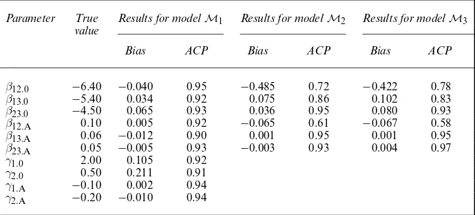
Table 1 shows the results of the simulation study. Looking at the bias and the actual coverage percentage (ACP) of estimated 95% confidence intervals, model M1 seems to have a better
overall performance than the other two models. An exception is the estimation ofβ13:A, where
modelM1induces a larger bias. The ACPs for modelM1are slightly less than their nominal
value. This may be caused by the sample size that is too small to fulfil the requirements of the asymptotic properties with respect to the maximum likelihood estimation. The performance of modelsM2 andM3 seems similar. These models induce severe bias in the estimation of
Table 1. Results for the simulation study with sample sizenD200 and 400 replications†
Parameter True Results for modelM1 Results for modelM2 Results for modelM3
value
Bias ACP Bias ACP Bias ACP
β12:0 −6.40 −0.040 0.95 −0.485 0.72 −0.422 0.78
β13:0 −5.40 0.034 0.92 0.075 0.86 0.102 0.83
β23:0 −4.50 0.065 0.93 0.036 0.95 0.080 0.93
β12:A 0.10 0.005 0.92 −0.065 0.61 −0.067 0.58
β13:A 0.06 −0.012 0.90 0.001 0.95 0.001 0.95
β23:A 0.05 −0.005 0.93 −0.003 0.93 0.004 0.97
γ1:0 2.00 0.105 0.92
γ2:0 0.50 0.211 0.91
γ1:A −0.10 0.002 0.94
γ2:A −0.20 −0.010 0.94
β12:0,β13:0andβ12:A. The models underestimate the risk of moving from state 1 to state 2 and
overestimate the risk of moving from state 1 to state 3—a bias that is absent for modelM1.
Even though the simulation study is limited in scope, it is clear that the presence of non-ignor-able missing states can lead to biased inference when the missing data mechanism is ignored in the multistate analysis.
5. Application
First we briefly discuss the Medical Research Council ‘Cognitive function and ageing study’ (CFAS) (Brayneet al., 2006). Next the three-state illness–death model will be defined where individuals are in state 2 when they have experienced one or more strokes and in state 1 if they have never had a stroke. This model was discussed in the previous sections. It will be denoted byM1and it includes the modelling of non-ignorable missing states. We shall estimate healthy
LE, which is defined as the remaining years of life spent stroke free.
As in Section 4, modelM1will be compared with two other models:M2is an MAR model
and forM3we ignore all intermittently missing states and estimate a complete-data model from
the observed states only.
5.1. Medical Research Council ‘Cognitive function and ageing study’
The Medical Research Council CFAS is a population-based longitudinal study of cognition and health in the older population of England and Wales. Interviews were conducted in five centres in England and Wales: Oxford, rural Cambridgeshire, Nottingham, Gwynedd and Newcastle. The study was designed to have 2500 individuals in each centre. There were 13 004 individuals who undertook the baseline interview in 1991 and since then they have had up to eight inter-views in the period 1991–2004. All individuals were aged 65 years and above at baseline, and all deaths up to the end of 2005 have been included. The time between interviews varies between and within individuals and the number of interviews is not fixed. The last observed state of an individual at the end of December 2005 is either death or censored and does not count as an interview.
Of interest are LE free from stroke and total LE. In what follows we describe and analyse the data from the Newcastle centre with 2512 individuals. At baseline there are 187 individuals with severe cognitive impairment. For this group, information on stroke history is missing or potentially unreliable. Although missing states at baseline can be incorporated in our model, the reliability of observed states poses problems that fall outside the scope of this paper. We therefore restrict our analysis to individuals who are not cognitively impaired at baseline. This also make sense clinically. Stroke is a potential cause of cognitive impairment and hence the stroke prevalence may not be estimated well for the cognitively impaired. Of the remaining 2325 individuals, four have a missing state at baseline. We removed these individuals from the data as modelling missing the baseline state for such a small group is not worthwhile. Hence there are 2321 individuals (880 men; 1441 women) in the analysis.
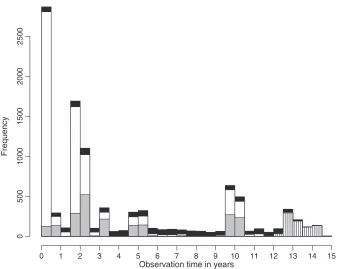
Fig. 1 provides information on the observation times for the four states. The CFAS had planned follow-up for all individuals at years 0, 2 and 10. Additional interviews were under-taken on selected individuals at years 1, 3, 6 and 8. These individuals are identified at previous interviews and hence missing interviews are easily identified.
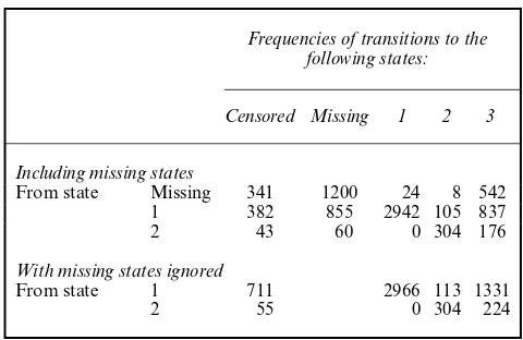
Table 2 presents frequencies of observed transitions between the states in the CFAS when missing states are included and when missing states are removed. Note that there are no transi-tions from state 2 to state 1. There are quite a large number of missing states and Table 2 shows that there are also many missing states that are followed by a missing state, i.e. there are 1200 transitions from a missing state to a missing state. In the CFAS, individuals who refused one interview are not allowed to be recontacted owing to ethical constraints. The figures in the second part of Table 2 can partly be derived from the first part: 2966=24+2942 and 113=8+105. It is, however, only given the second part that it becomes clear that 224−176=48 out of the 542 transitions from a missing state to state 3 are due to missing states in between an observed state 2 and observed death. Consequently, 542−48=494 transitions from a missing state to the death states are due to individuals with one or more missing states between an observed state 1 and observed death.
In general, a missing state is not a complication for a continuous time model. The model allows for varying times between interviews. If an individual misses an interview for unrelated reasons, then that is not a violation of model assumptions. However, if an individual misses an interview because he or she recently had a stroke, then the missing state is non-ignorable and if we ignore this scenario we could bias the estimates. Another problem with ignoring missing states is that the approximation to the time dependence of the intensities becomes more coarse.
Observation time in years
Freq
u
ency
0 1 2 3 4 5 6 7 8 9 10 11 12 13 14 15
0
5
00
1000
1500
2000
2500
Table 2. Frequencies of observed transitions between the states in the CFAS when missing states are included and when missing states are ignored
Frequencies of transitions to the following states:
Censored Missing 1 2 3
Including missing states
From state Missing 341 1200 24 8 542 1 382 855 2942 105 837 2 43 60 0 304 176
With missing states ignored
From state 1 711 2966 113 1331 2 55 0 304 224
For example, if the sequence is given by xt1,xt2,xt3,xt4=1,·,·, 3 and the missing states are
ignored, then the time dependence of the intensities in.xt1,xt4] is approximated by using age at .xt1+xt4/=2, whereas, if the missing states are not ignored, the time dependence is approximated by using age at.xt1+xt2/=2,.xt2+xt3/=2 and.xt3+xt4/=2.
5.2. Analysis
Time in the three-state model is the time since baseline in months. States of individuali are observed at timestijforj=1, . . . ,Mi, whereti1=0, andMi−1 is the number of planned
inter-views for individuali, and the state attMi is either censored or the death state. The model for the baseline state is given by
log.θi/=α0+αAAgei.ti1/+αSSexi+αEEducationi: .6/
To model possible time-dependent transition intensities, age in years is added as a time-dependent covariate in the log-linear model for the intensities. For interval.tij,ti,j+1],j∈{1, . . . ,Mi−1},
the model for the intensities and the probability of an observed state are given by
log{qrs.tij/}=βrs:0+βrs:AAgei{.tij+ti,j+1/=2}+βrs:SSexi+βrs:EEducationi,
logit{p1.ti,j+1/}=γ1:0+γ1:AAgei.ti,j+1/+γ1:SSexi+γ1:EEducationi+γ1:R1.Rtij=0/, .7/
logit{p2.ti,j+1/}=γ2:0+γ2:AAgei.ti,j+1/+γ2:SSexi+γ2:EEducationi+γ2:R1.Rtij=0/: .8/
Age in the models is centred by subtracting 78.5 years. Sex and Education are dummy variables (men≡1, more than 9 years of full-time education≡1). Note that age as a covariate for the piecewise constant intensities is evaluated midway through the interval.
The selection modelM1that includes the three-state model and the model for the missing
states is estimated by maximizing the log-likelihood in the programming environment R (R Development Core Team, 2008) by using the general purpose optimizeroptim. Withinoptim
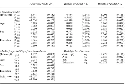
Table 3. Parameter estimates (with standard errors in parentheses)
Results for modelM1 Results for modelM2 Results for modelM3
Three-state model
(Intercept) β12:0 −6.441 (0.152) −6.454 (0.144) −6.294 (0.146)
β13:0 −5.401 (0.055) −5.403 (0.052) −5.295 (0.052)
β23:0 −4.534 (0.101) −4.539 (0.103) −4.420 (0.097)
Age β12:A 0.103 (0.016) 0.078 (0.018) 0.065 (0.018)
β13:A 0.062 (0.007) 0.070 (0.006) 0.065 (0.006)
β23:A 0.050 (0.009) 0.046 (0.010) 0.039 (0.010)
Sex β12:S 0.272 (0.193) 0.377 (0.195) 0.274 (0.200)
β13:S 0.308 (0.080) 0.296 (0.075) 0.266 (0.075)
β23:S 0.388 (0.122) 0.396 (0.127) 0.332 (0.126)
Education β12:E 0.345 (0.225) −0.045 (0.228) −0.168 (0.236)
β13:E −0.395 (0.124) −0.256 (0.093) −0.254 (0.090)
β23:E 0.180 (0.137) 0.123 (0.154) 0.067 (0.155)
Models for probability of an observed state Model for baseline state
(Intercept) γ1:0 1.097 (0.056) (Intercept) α0 −2.475 (0.116)
γ2:0 1.305 (0.184) Age αA 0.036 (0.012)
Age γ1:A −0.014 (0.007) Sex αS 0.369 (0.165)
γ2:A −0.066 (0.020) Education αE −0.571 (0.213)
Sex γ1:S 0.288 (0.089)
γ2:S 0.569 (0.286)
Education γ1:E 0.430 (0.108)
γ2:E −0.533 (0.316)
1.Rtij=0/ γ1:R −5.057 (0.211) γ2:R −4.180 (0.394)
model and the parameters for the three-state model are assumed to be distinct and the models are estimated separately.
ModelM1has−2×log-likelihood=23 975.92, whereas the same model with the restriction
γ1:R=γ2:R=0 has−2×log-likelihood=26 252.87. This difference in the log-likelihood shows
that the model with unrestrictedγ1:Randγ2:R is better and that whether or not the previous
state was observed helps to estimate the probability of observing the current state.
Table 3 shows the parameter estimates. As expected, the effect of age on the transition intensi-ties is positive (β12:A,β13:A,β23:A>0) and men have an increased risk of a transition to stroke as
well as to mortality (β12:S,β13:S,β23:S>0). Estimated models (7) and (8) for the probabilities of
observing a state show that the older you are the more likely it is that your state is not observed and that this age effect is stronger for state 2 than for state 1. Estimated model (6) for the baseline state shows that the probability of having a stroke increases with age (αA>0).
To estimate LEs we use the piecewise constant approximation as explained in Section 3. Grid u1,u2, . . . ,uM for the trapezoidal rule is defined by using h=1 month. In what follows, the
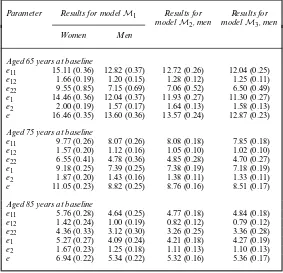
conditioning of the LEs onZ={z.t/|t0}is suppressed in the notation. Table 4 reports point estimates and standard errors that are derived from simulating model parameter uncertainty using the MLE (500 simulated parameter vectors). The mean of the point estimates in the sim-ulation can differ from point estimates that are calculated by using the MLE directly. This is due to possible skewness of the density of the LEs—even though the model parameters are simulated from a multivariate normal distribution. As an example, for men aged 65 years at baseline,e22is estimated to be 7.15 years by using the mean of the MLE simulations and 7.08
Table 4. Estimated LEs (with estimated standard errors in parentheses) for women and men given mean level of education
Parameter Results for modelM1 Results for Results for modelM2, men modelM3, men
Women Men
Aged 65 years at baseline
e11 15.11 (0.36) 12.82 (0.37) 12.72 (0.26) 12.04 (0.25)
e12 1.66 (0.19) 1.20 (0.15) 1.28 (0.12) 1.25 (0.11)
e22 9.55 (0.85) 7.15 (0.69) 7.06 (0.52) 6.50 (0.49)
e1 14.46 (0.36) 12.04 (0.37) 11.93 (0.27) 11.30 (0.27)
e2 2.00 (0.19) 1.57 (0.17) 1.64 (0.13) 1.58 (0.13)
e 16.46 (0.35) 13.60 (0.36) 13.57 (0.24) 12.87 (0.23)
Aged 75 years at baseline
e11 9.77 (0.26) 8.07 (0.26) 8.08 (0.18) 7.85 (0.18)
e12 1.57 (0.20) 1.12 (0.16) 1.05 (0.10) 1.02 (0.10)
e22 6.55 (0.41) 4.78 (0.36) 4.85 (0.28) 4.70 (0.27)
e1 9.18 (0.25) 7.39 (0.25) 7.38 (0.19) 7.18 (0.19)
e2 1.87 (0.20) 1.43 (0.16) 1.38 (0.11) 1.33 (0.11)
e 11.05 (0.23) 8.82 (0.25) 8.76 (0.16) 8.51 (0.17)
Aged 85 years at baseline
e11 5.76 (0.28) 4.64 (0.25) 4.77 (0.18) 4.84 (0.18)
e12 1.42 (0.24) 1.00 (0.19) 0.82 (0.12) 0.79 (0.12)
e22 4.36 (0.33) 3.12 (0.30) 3.26 (0.25) 3.36 (0.28)
e1 5.27 (0.27) 4.09 (0.24) 4.21 (0.18) 4.27 (0.19)
e2 1.67 (0.23) 1.25 (0.18) 1.11 (0.13) 1.10 (0.13)
e 6.94 (0.22) 5.34 (0.22) 5.32 (0.16) 5.36 (0.17)
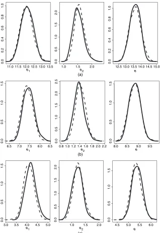
(4). It is only fore22 that the figures differ slightly—the densities of the other LEs are close to
symmetrical; see Fig. 2 for some of these densities.
In Section 3.2, the Metropolis algorithm was proposed as an alternative simulation method to estimate the variance of the LEs. We ran four sequences each of which contained 10 000 sim-ulated parameter vectors. For the starting values of the sequences we chose the MLE plus some random noise. The proposal density was multivariate normal and the algorithm was designed such that the acceptance rate was around 40%. Running the Metropolis algorithm for modelM1
is computationally intensive given that there are 22 parameters to estimate.
We illustrate the results for the marginal and total LEs for men with mean education level. Fig. 2 shows the comparison with the MLE simulation for men aged 65, 75 and 85 years at base-line. The two methods produce similar results, which is reassuring with regard to the reliance on the asymptotic properties of maximum likelihood in the MLE simulation. For women the comparison (which is not reported) was similar. The MLE simulation estimated slightly wider densities (bigger variance) fore2, but numerically the differences were small.
To obtain the estimate for men aged 65 years there is a long period of extrapolation and small differences between methods will have an effect. As can already be inferred from the relatively low frequencies of observed transitions from state 1 to state 2 (Table 2), and from the relatively large estimated variance of the parameters for the transition intensityq12.t/(Table 3),
estima-tion ofe12ande2is subject to a relatively large variance. In general, the estimated LEs for the
11.0 11.5 12.0 12.5 13.0 13.5 at baseline with mean education level: a comparison between MLE simulation (- - - ) and the Metropolis algorithm ( )
5.3. Sensitivity analysis
The parameter estimates for models (7) and (8) rely heavily on model assumptions. This is often so in missing data analysis: values ofXtare only observed whenRt=1, so estimates are driven
by model assumptions rather than by evidence in the data (Little (1995), page 1115). To inves-tigate the robustness of the missing data models, we discuss a sensitivity analysis that considers alternative link functions and functional form for the effect of age.
Models (7) and (8) are logit models where the link function is defined by logit.p/= log{p=.1−p/}. An alternative is the probit model that is defined by probit.p/=Φ−1.p/, whereΦis the standard normal cumulative probability distribution. Another possibility is the complementary log–log-model defined by cloglog.p/=log{−log.1−p/}. By using alternative link functions and comparing results we can investigate—up to a certain extent—whether the models for the missing data are robust against misspecification of the link function.
Another sensitivity analysis is to investigate functional form for the effect of age in models (7) and (8), where the slope is assumed to be constant. The assumption can be tested by for-mulating a spline function that imposes piecewise constant slopes with possible slope change at so-called knots; see, for example, Greene (2002). For age in years, we choose knotsg1, . . . ,g5=
71, 77, 83, 89, 95 and extend models (7) and (8) by adding covariates1.Agegk/.Age−gk/with
regression effectδk, fork=1, . . . , 5. (In the implementation, we took the centring of age into
account.) Another way to investigate functional form for the effect of age is to work with age categories. This can be used to investigate the assumption in models (7) and (8) that the effect of age is linear. The models were adapted by replacing the covariate age by five dummy variables for the categories 71–77, 77–83, 83–89, 89–95 andolder than95 years, and by using the category
younger than71 years as reference category.
The Akaike information criterion AIC can be used to investigate the alternatives formulated above. For modelM1with the logit models we obtain AIC=23 997. Using the probit link we
obtain AIC=24001 and, using the cloglog-link, AIC=23 994. Using spline regression, AIC =24 026. Since modelM1is nested in the model with the splines, the models can be compared
by using the likelihood ratio test: the difference in minus two times the log-likelihood is 13.55, which is not significant (p-value 0.19). Using the dummy variables for age, AIC=24 021. The AICs for the models with different link models are similar, and the AICs for the spline regres-sion and the regresregres-sion with the dummy variables show that these extenregres-sions do not yield better models.
More relevant is to see how estimated LEs change across the different specifications. Because of the extrapolation, if there are differences, they will be most pronounced in the LEs of individuals aged 65 years old at baseline. Both for the probit model and for the cloglog-model, absolute differences for LEs for women and men are all smaller than 0.1 when compared with the results in Table 4. Also, for the spline regression and the regression with the dummy variables for age, absolute differences for LEs for women and men are smaller than 0.1.
The above summary shows that the estimation of the LEs is robust across some of the possi-ble alternative specifications of the missing data model. Completely ignoring the missing data, however, does have a relevant effect on the estimation of LEs. This will be shown in the next section.
As stated at the end of Section 3.1, even though in some cases it is clear that the missing state is state 2, this state is not imputed before data are analysed. For the CFAS data at hand this is crucial. If we impute each of the 60 missing states of which we know that it must be state 2, selection modelM1as formulated in the previous section is difficult to estimate: for
the variance cannot be estimated as the Hessian is not positive definite. By using the restriction γ2:R=0, the model can be fitted, but estimated standard errors for submodel (8) are huge and
hamper further statistical inference. This shows that, by not imputing these specific missing states, we maintain information about the missing data mechanism that is needed to estimate modelM1.
5.4. Comparison with other models
In addition to the selection modelM1, modelsM2 and M3 were introduced in Section 4.
In what follows we compare the results for the three models with regard to the CFAS data. Although Section 4 showed that the models may yield different results, the true mechanism at work in the CFAS data is unknown as is how differences between parameter estimates affect estimation of LEs. We also consider the comparison betweenM1and Cox regression models
(Cox, 1972).
ModelM2can be fitted to the CFAS data without any changes and data for modelM3can
be derived from the CFAS data by deleting all the intermittently missing states. Table 2 presents frequencies of observed transitions between the states in the CFAS when missing states are removed.
Parameter estimates for the modelsM2 andM3 are presented in Table 3. If we assess the
significance of the covariates by using univariate Wald tests, then we see that the three models differ in the estimation of the non-significant effects, especially for education. More education is associated with better survival and in that sense ˆβ13:Eagrees with our expectation. Butβ12:Eand
β23are difficult to identify as is indicated by the relatively large standard errors. This may be due
to the relatively small number of individuals who are observed in state 2. In our data analysis, there is no clear association between the risk of stroke and education. For the significant effects, point estimates are similar although they differ. The biggest difference is for the effect of age on the intensity of moving from state 1 to state 2 (β12:A). The increase of this effect follows the
increase of the extent to which we model the missing states: 0.065 in modelM3, 0.078 in model
M2and 0.103 in modelM1. Since age increases for all individuals during follow-up, this means
that modelling the missing states leads to a higher estimated risk of a transition from state 1 to state 2.
Reported estimated standard errors in Table 3 show a pattern: the precision of the esti-mation of covariate effects for the transitions from state 1 to state 2 and for the transitions from state 2 to state 3 is highest for model M1. This concurs with the results in the
sim-ulation study where the means of the estimated standard errors (which are not reported in Table 1) showed that the selection model has a higher precision than the other two mod-els with regard to the effect of age on transitions from state 1 to 2 and for state 2 to 3. By modelling possible non-ignorable missing states, the probability that a latent state is state 2 is larger ( ˆγ2:0>γˆ1:0) and hence more covariate information is used to estimate the effects
for transitions to or out of state 2. Nevertheless, the differences in standard errors in Table 3 are small, and for some quantities modelsM2andM3are more efficient thanM1;
see, for example, interceptβ12:0and effectβ13:S. Overall, combining the data analysis with the
simulation study, the gain of modelling non-ignorable missing states is more about bias than precision.
As was to be expected, estimates for those aged 65 years differ the most. This is due to the extrapolation—differences between the models become more apparent under extrapolation. The largest difference is fore11, where modelM1estimates 12.85 (0.37) andM3estimates 12.04
(0.25). Looking at the point estimates, modelM2is an intermediate model, often producing
estimates that are in between the estimates ofM1andM3. For the younger ages, modelM1
estimates higher LEs. For these ages, a missing state is less likely to be state 2 according toM1
(Table 3: ˆγ2:A<0). As a consequence, the possibility of a trajectory from an observed state
1 via a latent state 2 is less likely and mortality decreases as state 2 is associated with poorer survival.
In general, the comparison of a three-state model such as model M1 with a Cox
regres-sion model is of limited use. But here the idea is to fit two Cox models—one for each baseline state—and to compare survival estimated by the Cox models with survival estimated by the three-state model. This does not provide information on the risk of a stroke or on healthy LE, but it is a way to validate part of the three-state model: if there is not too much censoring, then estimated survival should be similar (see Sianniset al.(2007)). Of course, this is only a comparison between models and as such not a goodness-of-fit test. Given that observation times vary within and between individuals and that age is used as a time-dependent variable, we cannot apply Pearson-type goodness-of-fit tests as described in Aguirre-Hernández and Fare-well (2002) and Titman and Sharples (2008).
Using the packagesurvivalin R, we fitted two Cox models with covariates age, sex and education as defined for modelM1. Age as a time-dependent variable was dealt with by
rear-ranging the data such that every individually observed time interval is a record in the data. This is thestart–stopformat; see, for example, Venables and Ripley (2002), section 13.4. An event is defined as death and age within each record is age midway through the corresponding time interval.
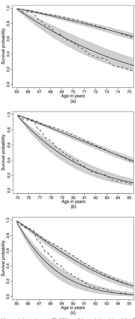
Fig. 3 depicts the results for men with mean education. For modelM1, we used a
piece-wise constant approximation to estimate survival for an individual with covariates specified at baseline. This is the same approximation as used in the estimation of the LEs. Given time grid u1,u2, . . . ,uM andh=1 month, survival at timeujfor an individual in statesat baseline was
estimated by 1− ˜P.u1,uj/[s, 3], whereP˜.u1,uj/=P.u1,u2/P.u2,u3/×. . .×P.uj−1,uj/. The
95% confidence intervals were derived from simulating model parameter uncertainty by using the MLE. For 500 simulated parameter vectors, survival was estimated and 95% confidence intervals were derived by using percentiles. For estimating survival given the Cox model, we used the same grid specification and used the functionsurvfitwith the optionnewdata(see Venables and Ripley (2002), section 13.4).
For men in state 1 at baseline, the two models estimate similar survival. The Cox model will always overestimate survival as it does not—for censored deaths—take into account a possible trajectory via state 2. For individuals in state 1 at baseline, 35% of the deaths are censored. (For individuals in state 2 at baseline, 11% of the deaths are censored.)
For men in state 2 at baseline, the two models estimate different survival for the older men —noticeably in the first half of the follow-up. This difference is partly due to left censoring. The Cox model analyses data from men who were in state 2 at baseline. ModelM1analyses in
65 66 67 68 69 70 71 72 73 74 75
0.0
0.2
0.4
0.6
0.8
1.0
Age in years
Survival probability
75 76 77 78 79 80 81 82 83 84 85
0.0
0.2
0.4
0.6
0.8
1.0
Age in years
Survival probability
85 86 87 88 89 90 91 92 93 94 95
0.0
0.2
0.4
0.6
0.8
1.0
Age in years
Survival probability
(a)
(b)
(c)
6. Conclusion
To take into account possible non-ignorable missing values, we fitted a selection model to the longitudinal data from the Medical Research Council CFAS. The selection model encompasses a continuous time three-state model to describe stroke history, and a missing data model to describe missing values. The model can be seen as an extension of the selection model in Cole
et al.(2005). Our model allows for right censoring and, by modelling time continuously, exact death times are taken into account. The selection model can be used to estimate stroke-free LE. The goodness of fit was checked graphically by comparing model-based survival with the survival estimated by the semiparametric Cox regression model.
Whether or not missing states are taken into account has an effect on the estimates of LEs. Modelling the missing states as non-ignorable leads to higher estimated stroke-free LE for men aged 65 years and to lower estimated stroke-free LE for the men aged 85 years.
The analysis is restricted to individuals in Newcastle who are not severely cognitively impaired at baseline. This means that estimated LEs are a little higher than expectancies for the whole population in Newcastle. Reported total LEs are below the national UK average, but this is specific to Newcastle and in line with reported estimates elsewhere; see, for example, Matthews
et al.(2006).
There are many ways in which informatively missing data can be ignored. The MAR model M2in this paper is rather specific—other MAR models are possible. The comparison between
modelM2and the selection modelM1is not meant as a general comparison between MAR
and missingness not at random models. A comparison which in general would not be very useful as every fit to observed data, obtained by using a missingness not at random model is exactly reproducible from an MAR model (Molenberghs and Kenward (2007), theorem 19.2). ModelM1relies on model assumptions that cannot be linked to evidence in the data. For this
reason, a sensitivity analysis was conducted to investigate functional form of the missing data model.
An issue that is not discussed in this paper even though it is quite common (and important) in longitudinal data analysis is missing values of covariates. There is no direct extension of our model to take into account missing covariate data. Since the model as-sumes covariates values to be fixed values, taking into account missing values of a covariate means introducing a distribution for the covariate—an exercise that is beyond the scope of this paper.
The model presented is flexible. It can be applied to data with more than three states and to data with backward transitions. The log-linear regression for the intensities makes it possible to model cohort effects by including calender year as a covariate, or to investigate risk factors that are associated with poor survival. The model is also intended as an alternative to the discrete time modelling that is implemented in the software IMaCh (Lièvreet al., 2003). IMaCh has been used in research on healthy LEs (see, for example, Jaggeret al.(2007) and Lièvreet al.(2008)), but the software always assumes that recovery from a disease or disability state is possible. In addition, modelling of non-ignorable missing values is not yet possible in IMaCH.
Acknowledgements
References
Aalen, O. O., Farewell, V. T., De Angelis, D., Day, N. E. and Gill, O. N. (1997) A Markov model for HIV disease progression including the effect of HIV diagnosis and treatment: application to AIDS prediction in England and Wales.Statist. Med.,16, 2191–2210.
Aguirre-Hernández, R. and Farewell, V. T. (2002) A Pearson-type goodness-of-fit test for stationary and time-continuous Markov regression models.Statist. Med.,21, 1899–1911.
Albert, P. S. and Follmann, D. A. (2003) A random effects transition model for longitudinal binary data with informative missingness.Statist. Neerland.,57, 100–111.
Brayne, C., McCracken, C. and Matthews, F. E. (2006) Cohort profile: the Medical Research Council Cognitive Function and Ageing Study (CFAS).Int. J. Epidem.,35, 1140–1145.
Cole, B. F., Bonetti, M., Zaslavsky, A. M. and Gelber, R. D. (2005) A multistate Markov chain model for longi-tudinal, categorical quality-of-life data subject to non-ignorable missingness.Statist. Med.,24, 2317–2334. Collett, D. (2003)Modelling Survival Data in Medical Studies, 2nd edn. London: Chapman and Hall–CRC. Commenges, D. (1999) Multi-state models in epidemiology.Liftime Data Anal.,5, 315–317.
Cox, D. R. (1972) Regression models and life-tables (with discussion).J. R. Statist. Soc.B,34, 187–220. Greene, W. H. (2002)Econometrics Analysis, 5th edn. New Jersey: Prentice Hall.
Izmirlian, G., Brock, D., Ferrucci, L. and Phillips, C. (2000) Active life expectancy from annual follow-up data with missing responses.Biometrics,56, 244–248.
Jackson, C. H., Sharples, L. D., Thompson, S. G., Duffy, S. W. and Couto, E. (2003) Multistate Markov models for disease progression with classification error.Statistician,52, 193–209.
Jagger, C., Matthews, R., Melzer, D., Matthews, F., Brayne, C. and MRC CFAS (2007) Educational differences in the dynamics of disability incidence recovery and mortality: findings from the MRC Cognitive Function and Ageing Study (MRC CFAS).Int. J. Epidem.,36, 358–365.
Kalbfleisch, J. and Lawless, J. F. (1985) The analysis of panel data under a Markov assumption.J. Am. Statist. Ass.,80, 863–871.
Kay, R. (1986) A Markov model for analysing cancer markers and disease states in survival studies.Biometrics,
42, 855–865.
Li, J., Yang, X., Wu, Y. and Shoptaw, S. (2007) A random-effects Markov transition model for Poisson-distributed repeated measures with non-ignorable missing values.Statist. Med.,26, 2519–2532.
Lièvre, A., Alley, D. and Crimmins, E. (2008) Educational differentials in life expectancy with cognitive impair-ment among the elderly in the United States.J. Agng Hlth,20, 456–477.
Lièvre, A., Brouard, N. and Heathcote, C. (2003) The estimation of health expectancies from cross-longitudinal surveys.Math. Popln Stud.,10, 211–248.
Little, R. J. A. (1995) Modeling the drop-out mechanism in repeated-measures studies.J. Am. Statist. Ass.,90, 1112–1121.
Little, R. J. A. and Rubin, D. B. (2002)Statistical Analysis with Missing Data, 2nd edn. New York: Wiley. Matthews, F. E., Miller, L. L., Brayne, C., Jagger, C. and Medical Research Council Cognitive Function and
Aging Study (2006) Regional differences in multidimensional aspects of health: findings from the MRC cogni-tive function and ageing study.BMC Publ. Hlth,6.
Molenberghs, G. and Kenward, M. G. (2007)Missing Data in Clinical Studies. Chichester: Wiley.
Molenberghs, G., Kenward, M. G. and Lesaffre, E. (1997) The analysis of longitudinal ordinal data with nonrandom drop-out.Biometrika,84, 33–44.
Norris, J. R. (1997)Markov Chains. Cambridge: Cambridge University Press.
Putter, H., Fiocco, M. and Geskus, R. B. (2007) Tutorial in biostatistics: competing risks and multi-state models. Statist. Med.,26, 2389–2430.
R Development Core Team (2008)R: a Language and Environment for Statistical Computing. Vienna: R Foun-dation for Statistical Computing.
Rubin, D. B. (1976) Inference and missing data (with discussion).Biometrika,63, 581–592.
Satten, G. A. and Longini, Jr, I. M. (1996) Markov chains with measurement error: estimating the ‘true’ course of a marker of the progression of human immunodeficiency virus disease (with discussion).Appl. Statist.,45, 275–309.
Siannis, F., Farewell, V. T. and Head, J. (2007) A multi-state model for joint modelling of terminal and non-terminal events with application to Whitehall II.Statist. Med.,26, 426–442.
Tanner, M. A. (1996)Tools for Statistical Inference. New York: Springer.
Titman, A. C. and Sharples, L. D. (2008) A general goodness-of-fit test for Markov and hidden Markov models. Statist. Med.,27, 2177–2195.
Van den Hout, A. and Matthews, F. E. (2009) A piecewise-constant Markov model and the effects of study design on the estimation of life expectancies in health and ill health.Statist. Meth. Med. Res.,18, 145–162.