2009
Technical Report on Information-Based Induc-tion Sciences 2009 (IBIS2009)
Observational Reinforcement Learning
Jaak Simm, Masashi Sugiyama, and Hirotaka Hachiya
∗Abstract: We introduce an extension to standard reinforcement learning setting called
observational RL (ORL) where additional observational information is available to the agent. This allows the agent to learn the system dynamics with fewer data samples, which is an essential feature for practical applications of RL methods. We show that ORL can be formulated as a multitask learning problem. A similarity-based and a component-based multitask learning methods are proposed for learning the transition probabilities of the ORL problem. The effectiveness of the proposed methods is evaluated in experiments of grid world.
1
Introduction
Recently, there is an increasing interest for methods of planning and learning in unknown and stochastic environments. These methods are investigated in the field of Reinforcement Learning (RL) and have been applied to various domains, including robotics, AI for computer games, such as tetris, racing games and fight-ing games. However, one of the main limitfight-ing factors for RL methods has been their scalability to large en-vironments, where finding good policies requires too many samples, making most RL methods impractical.
1.1
Transfer Learning in RL
One of the approaches for solving the scalability problem is to reuse the data from similar RL tasks by transferring data or previously found solutions to the new RL task. These methods have been a focus of the research lately and are called transfer learning
methods. The transfer learning methods can be sepa-rated into value-based and model-based transfer learn-ing methods, dependlearn-ing on what is belearn-ing transferred between the RL tasks.
In value-based transfer learning the value functions of previously solved RL tasks are transferred to the new task at hand. A popular approach for trans-ferring value functions is to use the previously found value functions as initial solutions for value function of the new RL task. These methods are called starting-point methods, for example see the temporal-difference learning based approach by Tanaka and Yamamura [4] and a comparative study of these methods by Taylor et al. [5]. For successful transfer, a good mapping of states and actions between the RL tasks is required. When a poor mapping is used the transfer can result in worse performance than doing the standard rein-forcement learning without a transfer.
∗Department of Computer Science, Tokyo Institute of
Tech-nology, Tokyo, Japan
On the other hand, model-based transfer learning methods transfer the transition models and reward models from the solved RL tasks to new RL tasks. Sim-ilarly to the value-based transfer, the mapping between states and actions of the learned RL tasks and the tar-get RL task is required. However, the requirements for the mapping are weaker than those in the case of value-based transfer and, thus, the transfer is also pos-sible between less similar tasks. The reason is that the transition model and reward model only depend on a single transition from the current state whereas the value function depends on a sequence of rewards (and thus transitions) starting from the current state. This difference can be seen from an example of transferring knowledge from a previous task where the agent is able to obtain a big positive reward after opening the door and moving around in the room behind the door. How-ever, if the new RL task gives a negative reward after the agent enters the room, the value-based transfer is not useful, probably even worsening the performance. On the other hand, model-based transfer could trans-fer the knowledge that the opening of the door allows to enter the room and if the agent has already learned that the room contain negative rewards in the new task it can infer the negative value of the actions that open the door and enter that room. In summary, the advan-tage of model-based transfer over value-based transfer is in cases where actions in different tasks have similar results, e.g., the same action opens the door, but the value of the action is different between the tasks.
A model-based transfer method called was proposed by Wilson et al. [6] that successfully estimates the probabilistic prior of tasks. If the model of the new task is similar to previously encountered tasks, the data from the previous tasks can be used to estimate the transition and reward model for the new task. Thus, the new task can be learned with fewer samples. A similar approach has also been applied to partially observable environments [2].
least one initial task. That is “previous tasks”, which are used in transfer learning of new tasks, should have been learned with sufficient accuracy. If the tasks have large state spaces, then the initial learning will require a huge amount of data, which is not realistic. This kind of setting where the tasks are ordered is called
transfer learning. In contrast, multitask learning is a setting where there is no initial task and all tasks are solved simultaneously. Another issue with the above reviewed methods is that the advantage of transferring between large RL tasks is problematic because a good mapping between them is usually not available.
1.2
Proposed Observational Idea
To tackle the above mentioned problems we propose a setting where the sharing does not occur between dif-ferent RL tasks but between difdif-ferent regions (parts) of the same RL task. This is accomplished by allowing the agent to access additionalobservationaldata about the regions of state-action space of the RL task. The usefulness of the observational data is that it identifies the regions of the task that participate in the multi-task learning. Moreover, the strength of the sharing between different regions depends on the similarity of their observations. The more similar the observations are, the stronger the sharing is. This kind of obser-vational data is often available in practice, e.g., in the form of camera data or sensor measurements.
A motivating example for our observational frame-work is a mobile robot moving around on a ground, where there are two types of ground conditions: slip-pery and non-slipslip-pery. The robot knows its current location and thus, can model the environment using a standard Markov decision formulation, predicting the next location from the current location and the move-ment action (e.g., forward and backward). However, if the robot has access to additional sensory information about the ground conditions at each state, it could use that additional observation to share the data between similar regions and models of the environment more efficiently even when only a small amount of transi-tion data is available. We call this kind of RL setting
Observational RL.
In our observational setting there is no order for solv-ing the tasks, meansolv-ing that all regions are solved simul-taneously, i.e., as a multitask learning setup. Addition-ally, since the sharing takes place between regions of the whole problem, the mapping is essentially between smaller parts of the problem. Therefore, the problem of finding a good mapping is often mitigated.
In our proposed setting, the model-based sharing is more natural than the value-based sharing, as the value of the states often depends on the global location of the region, and thus the value of similar regions is not expected to be same. In the mobile robot example described above, the probabilities of moving forward
would be similar in locations with similar ground con-ditions, but the value of going forward in these loca-tions depends on where the robot makes a transition to after executing the forward action. For this reason, from here we only focus on the model-based multitask learning in the setting of ORL.
1.3
Outline
In the next section we formally introduce the setting of ordinary RL. The notions of observations and sim-ilarity will be formalized in Section 3. After that we propose two methods for solving the Observational RL problem in Section 4. Their performance is evaluated experimentally in Section 5. Finally, we conclude in Section 6.
2
Ordinary RL
The goal of reinforcement learning is to learn optimal actions in unknown and stochastic environment. The environment is specified as a Markov Decision Problem (MDP), which is a state-space-based planning problem defined byS,PI,A,PT,Randγ. HereS denotes the set of states,PI(s) defines the initial state probability,
A is the set of actions, and 0≤γ <1 is the discount factor. The state transition functionPT(s′|s, a) defines the conditional probability of the next state s′
given the current statesand actiona. At each step the agent receives rewards defined by functionR(s, a, s′
)∈R. The goal of RL is to find a policy π: S → A that maximizes the expected discounted sum of future re-wards when the transition probabilitiesPT and/or the reward function R is unknown. The discounted sum of future rewards is∑∞t=0γtrt, wherert is the reward received at step t. In this paper we focus on the case where the transition probabilities are unknown, but the reward function is known, due to space constraints. The extension of the proposed methods to an unknown reward function is straight-forward.
3
Observational RL
In this section we formulate the setting of Observa-tional RL (ORL). For better understandability, we first start with a simpler framework that already includes the main idea. Then, later extend it to a more general setting.
3.1
Basic Idea
The Observational RL setting extends the ordinary RL setting by allowing the agent to access additional observational information about the state-action space. For the basic case, consider that the agent has obser-vations about each state 1. This means that for each
1
state s ∈ S the agent has some observation o ∈ O, whereOis the set of observations. Thus, formally the observational information can be defined as a function
φ(s) ∈ O mapping each state to its observation. For example, in the case of the mobile robot these obser-vations could be sensor measurements about ground conditions at each location.
The general idea of ORL is to use these additional observations for speeding up the learning, thus, requir-ing fewer samples to find good policies. ORL will be ef-fective if the states that have similar observations have similar transition structure. If the transition structure has nothing in common applying ORL-based methods will not be able to improve the performance. On the other hand, if similar observations imply similar transi-tion structure, then ORL-methods should have strong advantages.
The current paper focuses on the model-based RL approach [3], which consists of following two steps:
1. Estimate the transition probabilities PT(s′|s, a) using transition data.
2. Find an optimal policy for the estimated tran-sition model by using a dynamic programming
method, such as value iteration.
More specifically, the transition data consists of, pos-sibly non-episodic2, samples {(s
t, at, s′t)}Tt=1, wherest and at correspond to the current state and action of thet-th transition ands′
t is the the next state. Thus, the idea is to use observational data expressed byφto have more accurate estimates of the transition proba-bilitiesPT.
To take advantage of observational information we have to require that the agent assumes a common pa-rameterization for the transition models for all states. In other words, transition probabilities for all states are modelled with the same parametric formPT(s′|s, a;βs) whereβsis the parameter for the transition model for state s. For example, in the case of discrete MDPs, we can use a multinomial parameterization. This com-mon parameterization implicitly defines the mapping between the actions and next states of different states. Thus, it is similar to the mappings used in other trans-fer learning methods discussed in Section 1.1.
Similarly to other transfer learning methods the choice of mapping (in the case of ORL the choice of the parameterization) greatly affects the performance. Use of improper parameterization will negate all ad-vantages of data sharing and could even worsen the performance, depending on what method is used for solving the ORL problem.
Next we formalize the ORL framework that extends the described basic idea.
2Non-episodic means that there is no requirement that the
next state of thet-th transition sample (i.e.,s′
t) has to equal to
the starting state of the (t+ 1)-th transition sample (i.e.,sn+1).
3.2
Formulation of ORL
In the previous formulation the observations were just connected to single states. It is useful to extend the formulation by connecting the observations to re-gions (i.e., subsets) of the state-action spaceS×A. Let
udenote a region an observation is connected to. We calluan observed region and as it is a subset of state-action space u ⊂ S×A. Thus, the basic ORL idea described above was just a special case when u ∈ S. There are two motivations for this extension. Firstly, it allows us to work with structural problems where one observation is connected to several states, e.g., a manipulation task of various objects by a robotic arm, where an observation is connected to an object, and thus to all states involved in the manipulation of that object. Secondly, this extension means that the obser-vations are now also connected to actions. This allows one to have different observations for different actions and the sharing can depend on actions. For example, in the mobile robot case the movement actions (for-ward and back(for-ward) could participate in the sharing, whereas some other actions, such as picking up an ob-ject, could be left out from the sharing.
Now the observations function φ: U →O whereU
contains all observed regions. If there are N obser-vations then, the observational data is {(un, on)}Nn=1
where observationon∈O corresponds to regionun ⊂
S ×A. In this case the set of observed regions is
U ={un}Nn=1.
Additionally, we require that states can belong at most to a single observed region, this means that
ui∩uj = ∅, for i ̸= j. However, there is no require-ment that all state-action pairs belong to an observed region. The state-action pairs that do not belong to any observed region do not benefit from the observa-tional information. This extension allows the agent to consider models where all regions of the state-action space are not equipped with observations or certain parts of the state space are different, e.g., there is a maze with corridors and rooms and the agent only has observations about the rooms.
Next we propose two methods for solving the ORL problem.
4
Proposed Methods
First of the methods is based on the similarity idea and the second one comes from the mixture-of-components multitask learning ideas.
4.1
Similarity-based ORL
the single task estimation of maximum (log) likelihood for observed regionu
ˆ
βu= argmax βu
∑
(s,a,s′)∈Du
logPT(s′|s, a;βu), (1)
whereDu is a set of transition data from observed re-gionu. A straight-forward extension of the single task estimation (1) is to add data from other tasks and weight them according to the similarity of the other tasks to the current task at hand. This can be ex-pressed by
ˆ
βu= argmax βu
∑
v∈U
∑
(s,a,s′)∈Dv
ku(v) logPT(s′|s, a;βu),
(2)
where ku(v) ∈ [0,1] is the similarity of the observed region v to observed region u. Thus, data from ob-served regions that have high similarity ku(v) have a big effect on the estimation of the model of regionu. In the case of a mobile robot, consider the estimation of the model for a region of slippery statesu(e.g., an icy region). If the similarity functionku assigns high similarity to other regions of slippery states (e.g., other icy regions or wet regions) and a low similarity value for non-slippery states then the similarity-based ORL method will provide an accurate estimate forβu even if regionuhas few or no samples.
A practical option for the similarity function is to just use the Gaussian kernel between the observations of the regions, expressed as
ku(v) = exp(−∥φ(u)−φ(v)∥2/σ2), (3) where σ is the width of the kernel. This parameter could be chosen using cross-validation and it controls how much multitask effect distant tasks have on the current task at hand.
The only constraint onkuis that it should give value 1 for the region itself, i.e.,ku(u) = 1. No other proper-ties are required. Thus, we also allow non-symmetric and non-positive definite similarities.
One disadvantage of similarity-based ORL is it suf-fers from the curse of dimensionality if the observations are high-dimensional. In this case it means that all tasks will become dissimilar to each other due to the high-dimensionality of observations. Therefore, next we will introduce a more sophisticated method that is based on mixture-of-components, which uses a proba-bilistic framework to model the multitasking problem of ORL and thus could be expected to mitigate the above mentioned problem.
4.2
Component-based ORL
In this section we introduce a component-based mul-titask learning method for learning transition probabil-itiesPT(s′|s, a) for ORL.
Consider again the example of a mobile robot that is moving along a difficult terrain that has obstacles and varying ground conditions. The robot knows its loca-tion and speed at each step. That knowledge allows the robot to learn the state transition probabilities for each action. However, if the robot has access to additional observations about the states (using sensors or a cam-era), then using such observational information could allow the robot to estimate the transition probabilities in fewer samples than by just using robots location and speed.
Recall that in ORL the agent has access to obser-vations, i.e., the agent knows function φ(u)∈O. For example, for the mobile robot the set of observations could contain measurements about the ground type (e.g., gravel or tarmac) or visual information about the obstacles around a particular location. As already mentioned, in terms of multitask learning an observed regionu∈U is a task andφ(u) specifies its features.
Here we introduce the idea of component-based mul-titask learning where the role of task features is to a priori determine the component the task belongs to. Let there be M components, thenP(m|φ(u)) denotes the probability that the task uwith features φ(u) be-longs to the componentm(wherem∈ {1, . . . , M}).
Let (s, a) be a state-action pair and u∈U be such that (s, a)∈ u, then the sharing between elements of
U is formulated as a mixture of components for the transition probability:
PT(s′|s, a) = M
∑
m=1
PT(s′|s, a, m)P(m|φ(u)), (4)
where PT(s′|s, a, m) is the transition probability to states′ under componentmfor state-action pair (s, a)
and P(m|φ(u)) is the component membership proba-bility mentioned above. In the example of a mobile robot, these components would comprise of states that have similar transition dynamics, e.g., one component could be a group of states where a certain moving ac-tion fails due to difficult ground condiac-tions and another component represents states where the moving action succeeds.
Given the number of componentsM and data about transitions and observations, we want to find the max-imum likelihood estimate for (4). To do that we first need to assume a parametric form for its elements. The parameterized version of (4) is given by
P(s′
|s, a, β, α) = M
∑
m=1
P(s′
|s, a, βm)P(m|φ(u), α), (5)
estimation is tractable. The choice of parameterization forP(m|φ(u), α) depends on the type of observations,
O. For discrete observations an option is to use a Naive Bayes model:
P(m|o, α) =αm,0
K
∏
k=1
αm,k,ok, (6)
whereo is observation, i.e., o=φ(u) = (o1, . . . , oK)T.
Parameterαm,0controls the overall probability of
com-ponentmandαm,k,ok controls the probability of
com-ponentmfor regions whose observation’sk-th dimen-sion is equal to ok. Since parameters are multiplied together, the model assumes that each dimension in-dependently affects the component probability.
For continuous observations following parameteriza-tion can be used:
P(m|φ(u), α) =∑ exp(⟨αm, φ(u)⟩)
¯
m=1exp(⟨αm¯, φ(u)⟩)
, (7)
where φ(u) denotes the observation for u, αm ∈ RK, i.e., observations are K-dimensional real values, and
⟨·,·⟩ is inner product. This parameterization corre-sponds to multi-class logistic regression problem.
Because of its complicated form, the maximum like-lihood estimate for (5) cannot be found using straight-forward optimization. A standard approach doing maximum likelihood estimation on such problems is to use an EM-based method [1]. To do that we introduce a latent indicator variable
z∈ {0,1}M, (8)
which denotes the true component for u. Thus, only one of the elements ofzis equal to one and all others
are equal to zero. Usingzwe can rewrite the mixture
(5) as
P(s′
,z|s, a, β, α)
= M
∑
m=1
zmP(s
′
|s, a, βm)P(m|φ(u), α) (9)
= M
∏
m=1
[P(s′|
s, a, βm)P(m|φ(u), α)]zm
, (10)
where the summation form is transformed into a prod-uct form, which allows us to easily handle the log likeli-hood. This latent variable formulation allows us to use the EM algorithm for determining a maximum likeli-hood solution forβ andα.
The outline of the EM-method is
1. Start with initial values for parametersβ andα.
2. Calculate the posterior probabilities of the latent variables, given the parametersβandα(E-step).
1: KL-divergence of the estimated transition proba-bilities from the true model, for the slippery grid world experiment with2-dimensional observations. For each method the mean and standard deviation of its KL-divergence averaged over 50 runs are reported, for dif-ferent data sizes N = 50, N = 100, N = 150, and
N = 200. Bolded values in each column show methods whose performance is better than others using t-test with 0.1% confidence level.
Method N = 50 N = 100 Comp(1) 0.375±0.065 0.280±0.023 Comp(2) 0.373±0.102 0.177±0.036
Comp(3) 0.422±0.123 0.235±0.069 Comp(CV) 0.322±0.053 0.190±0.051
Sim(fixed) 0.369±0.046 0.207±0.022 Sim(CV) 0.338±0.028 0.211±0.023
Single task 1.686±0.004 1.628±0.006
(a)N= 50 andN= 100
Method N= 150 N = 200 Comp(1) 0.255±0.012 0.244±0.013 Comp(2) 0.117±0.034 0.080±0.034
Comp(3) 0.164±0.051 0.123±0.045 Comp(CV) 0.127±0.032 0.094±0.035
Sim(fixed) 0.153±0.015 0.125±0.010 Sim(CV) 0.162±0.021 0.132±0.014 Single task 1.576±0.008 1.526±0.009
(b)N= 150 andN= 200
3. Findβ andαthat maximize the expectation of the regularized data likelihood (M-step).
4. If the solution has converged stop, otherwise go to step 2.
Due to space restriction we leave out the details of E-step and M-step and only present the conclusions. E-step can be performed analytically by just applying the Bayes law. The M-step for transition models can be performed analytically for discrete and Gaussian models and M-step for observation-based component membership parameterαcan be effectively computed by convex optimization based methods.
We follow standard approach for implementing the EM method. This includes using several restarts to the EM procedure to avoid local optima and using cross-validation to choose the number of components (M).
5
Experimental Results
In this section we present experimental results from two simulated domains: grid world with slippery ground conditions.
5.1
Slippery Grid World
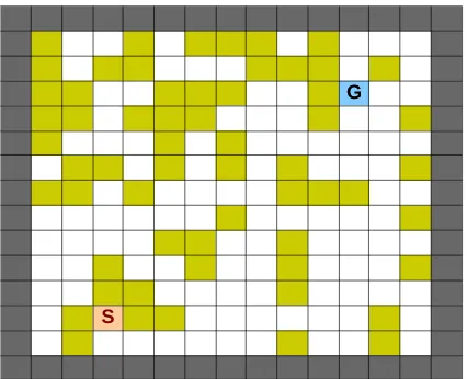
state space of the grid world is 15×15 and there are 4 movement actions: left, right, up and down. There are two types of states, one type is slippery, where all movement actions fail with probability 0.8, keeping the robot at the same spot and the other type is non-slippery having probability of failure 0.15. The goal of the agent is to reach the goal state from the initial state. An example of the grid world is shown in Figure 1. The goal of the robot is to reach the goal state denoted with “G” starting from bottom left state “S”. White squares are non-slippery and colored squares are slippery states. If the robot moves at the edge squares it receives a negative reward of−1 and is reset to the starting state. The robot receives reward +1 when it reaches goal state, after which it is again reset to the initial position. Other states do not give any reward.
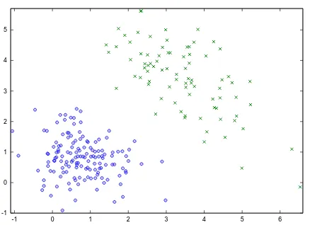
The observations about each state are two-dimensional real values of sensor measurements. The first dimension shows the measurement of the depth of the water layer covering the ground at that loca-tion and the second dimension the amount of loose gravel. Both measurements are noisy and for the experiments are generated randomly from two Gaus-sian distributions, one for slippery states and another for non-slippery states. The two Gaussians are quite separated, as can be seen from Figure 2.
The average performance over 50 runs for the component-based and the similarity-based ORL meth-ods is reported in Table 1. The table reports average KL-divergence values of the estimated transition prob-abilities from the true transition probprob-abilities. Meth-ods named ‘Comp(n)’ are component-based methods with n components. Thus, ‘Comp(1)’ actually just merges all observed regions as a unified task. The re-sults in Table 1 use transition data that is collected uni-formly over the state and action space, this allows us to compare the pure performance of different methods without the side effects of non-uniform data collect-ing policy. Secondly, in this experiment the methods used manually-chosen parameters to show the perfor-mance of the methods without the problem of choos-ing optimal parameters. For component-based meth-ods, ‘Comp(2)’ and ‘Comp(3)’, we manually chose the regularization parameter of the logistic regression to be 10−3. For similarity-based method ‘Sim(fixed)’ the
Gaussian kernel with a fixed widthσ= 2.5 was used. The single task method that does not use observations and ‘Comp(1)’ do not have any extra parameters.
Table 1 also reports the performance of methods using cross-validation(CV) for the choice of the pa-rameters. The ‘Comp(CV)’ is the component-based ORL that uses 5-fold CV to choose the regulariza-tion parameter for logistic regression from the set
{10−3,10−1,100}and the number of components.
Sim-ilarly, ‘Sim(CV)’ is the similarity-based ORL that uses 5-fold CV to choose the optimal width for the Gaussian kernel from the set{1.5,3.0,4.5,6.0,10.0}.
Firstly, we can use the performance of the unified
1: Mobile robot in a grid-world with slippery and non-slippery states. Robot starts from an initial state at bottom left denoted with “S” and has to reach the goal state “G”.
task (‘Comp(1)’) as a good comparison point in Ta-ble 1, because unifying all tasks is not expected to provide good results when a large number of samples are available. All ORL methods outperform the ‘Sin-gle task’ implying that the use of data sharing in this case is valuable, even with just 50 samples. As ex-pected the component-based method using 2 compo-nents ‘Comp(2)’ is performing the best overall with 100 or more samples. The performance of ‘Comp(3)’ and ‘Sim(fixed)’ is slightly worse than ‘Comp(2)’, but still clearly outperforming the unified task and single task methods, validating their usefulness in this exper-iment.
Also, as seen from Table 1 the cross-validation ver-sion of component-based method ‘Comp(CV)’ is per-forming almost as well as the best fixed parameter ver-sion. Actually in the case N = 50 the CV method is outperforming the fixed methods, because the regular-ization that was used in the fixed cases (10−3) is too
small, resulting in poor performance of the EM-based method, if only 50 samples are available. The effect of the regularization of logistic regression is depicted in Figure 3(a) for sample sizes 100 and 200. For both sample sizes if the regularization is not too big the component-based ORL has good performance.
Similarly, the ‘Sim(CV)’ method is very close to the fixed width case and the performance of similarity-based ORL is not very sensitive to the chosen Gaus-sian widths unless a too small width is chosen as seen from Figure 3(b). These results suggest that CV can be used for tuning the parameters of component-based and similarity-based ORL.
-1 0 1 2 3 4 5
-1 0 1 2 3 4 5 6
2: Distribution of observations for non-slippery (blue circles) and slippery (green crosses) states. The horizontal axis displays the measured water level and the vertical axis displays the measured amount of loose gravel for each state.
10−6 10−5
10−4 10−3
10−2 10−1
100 101
102 0
0.05 0.1 0.15 0.2 0.25 0.3 0.35
Regularization for logistic regression
KL−error
N=100 N=200
(a) Dependence of component-based ORL on the regularization of logistic regression.
0 1 2 3 4 5 6
0.1 0.2 0.3 0.4 0.5 0.6 0.7 0.8 0.9
Kernel width
KL−error
N=100 N=200
(b) Dependence of similarity-based ORL on Gaus-sian width.
3: Average KL-divergence from the true distribu-tion in slippery grid world tasks withtwo-dimensional
observations for sample sizesN = 100 and N = 200. The averages and standard deviations were calculated from 50 runs.
are quite close to the value of optimal policy, which is 0.799 in this task. The good performance of ‘Comp(1)’ is explained be the fact that in their nature the slippery and non-slippery states are similar, because all 4 ac-tions result in similar outcomes, just the probabilities of these outcomes differ.
2: Value of the the policy found by using the es-timated transition probabilities, for the slippery grid world experiment with 2-dimensional observations. For each method the mean and standard deviation of its value averaged over 50 runs are reported, for dif-ferent data sizes N = 50, N = 100, N = 150, and
N = 200. Bolded values in each column show methods whose performance is better than others using t-test with 0.1% confidence level.
Method N = 50 N = 100 Comp(CV) 0.716±0.054 0.746±0.023
Sim(CV) 0.715±0.036 0.749±0.021
Comp(1) 0.638±0.009 0.649±0.006 Single task −0.503±0.117 −0.370±0.179
(a)N= 50 andN= 100
Method N = 150 N = 200 Comp(CV) 0.754±0.016 0.757±0.018
Sim(CV) 0.756±0.005 0.757±0.004
Comp(1) 0.652±0.002 0.651±0.001 Single task −0.237±0.196 −0.102±0.179
(b)N= 150 andN= 200
5.2
Grid World with High-dimensional
Observations
We also tested the grid world example width high di-mensional observations. Now the observations were 10-dimensional. The first two dimensions were exactly the same as before, containing useful information about the states as depicted in Figure 2. The new 8 dimen-sions did not contain any information, i.e., the obser-vations for slippery and non-slippery states were gen-erated from the same distribution, which was a single 8-dimensional Gaussian with zero mean and identity covariance.
The results of high-dimensional grid world experi-ments for component-based and similarity-based ORL methods with CV are shown in Table 3. The sets of model parameters used by CV are the same as in the previous experiment. For comparison the results for ‘Comp(1)’ and ‘Single task’, are also presented in the table and as they do not use observations, we just re-port again their performance from the previous exper-iment.
Comparing Table 3 to Table 1 shows that the per-formance of both ORL methods is degraded compared to the problem with low-dimensional observation. As expected, the performance of the similarity-based ap-proach, ‘Sim(CV)’, has worsened more than the perfor-mance of the component-based approach, ‘Comp(CV)’. The similarity-based approach just slightly outper-forms the unified task ‘Comp(1)’ for sample sizes
3: KL-divergence of the estimated transition prob-ability from the true model, for the slippery grid world experiment with 10-dimensional observations. For each method the mean and standard deviation of its KL-divergence averaged over 50 runs are reported, for different data sizesN = 50, N = 100, N = 150, and
N = 200. Bolded values in each column show methods whose performance is better than others using t-test with 0.1% confidence level.
Method N= 50 N = 100 Comp(CV) 0.395±0.085 0.248±0.044
Sim(CV) 0.398±0.047 0.285±0.014
Comp(1) 0.375±0.065 0.280±0.023
Single task 1.686±0.004 1.628±0.006
(a)N= 50 andN= 100
Method N = 150 N= 200 Comp(CV) 0.190±0.054 0.140±0.039
Sim(CV) 0.244±0.014 0.222±0.012 Comp(1) 0.255±0.012 0.244±0.013 Single task 1.576±0.008 1.526±0.009
(b)N= 150 andN= 200
4: Value of the the policy found by using the es-timated transition probabilities, for the slippery grid world experiment with 10-dimensional observations. For each method the mean and standard deviation of its value averaged over 50 runs are reported, for dif-ferent data sizes N = 50, N = 100, N = 150, and
N = 200. Bolded values in each column show methods whose performance is better than others using t-test with 0.1% confidence level.
Method N = 50 N = 100 Comp(CV) 0.648±0.101 0.699±0.048
Sim(CV) 0.659±0.014 0.667±0.020
Comp(1) 0.639±0.011 0.649±0.005
Single task −0.508±0.121 −0.380±0.177
(a)N= 50 andN= 100
Method N= 150 N = 200 Comp(CV) 0.724±0.043 0.740±0.027
Sim(CV) 0.705±0.033 0.727±0.024
Comp(1) 0.652±0.002 0.651±0.001 Single task −0.279±0.192 −0.135±0.201
(b)N= 150 andN= 200
rather well and clearly outperforms other methods for
N = 150 andN = 200.
Table 4 shows the value of the policies that were found from the transition probabilities learned by dif-ferent methods for high-dimensional observations case. As expected, compared to the case of low-dimensional observations (see Table 2) both ORL methods have weaker performance. The component-based method slightly outperforms similarity-based method, signifi-cantly only forN = 100. This suggests that although
the KL-error of the similarity-based method is much higher than the component-based method, it still cap-tures useful structure in the transition probabilities re-sulting in almost similar performance in the grid world task.
In summary, both ORL methods show good perfor-mance in the grid world task and the curse of dimen-sionality has mild effect on their performance.
6
Conclusions
The results of the grid world task show that the pro-posed ORL framework is suitable in cases useful obser-vations are available about the state-action space. The two proposed method were shown to effectively employ the additional observations to speed up the learning of the transition probabilities.
Our next step is to apply the proposed methods to a more challenging task of object lifting by robotic arm where the robot has observations about the objects. Additionally, our future work is to investigate the re-lationship of ORL to the studies of Bayesian RL and Partially Observable MDP (POMDP).
[1] Christopher M. Bishop. Pattern Recognition and Machine Learning. Information Science and Statis-tics. Springer, 2006.
[2] Hui Li, Xuejun Liao, and Lawrence Carin. Multi-task reinforcement learning in partially observable stochastic environments. The Journal of Machine Learning Research, 10:1131–1186, 2009.
[3] Richard S. Sutton and Andrew G. Barto. Rein-forcement Learning. MIT Press, Cambridge, MA, USA, 1998.
[4] Fumihide Tanaka and Masayuki Yamamura. Mul-titask reinforcement learning on the distribution of MDPs. In Computational Intelligence in Robotics and Automation, 2003, volume 3, pages 1108–1113, July 2003.
[5] Matthew E. Taylor, Peter Stone, and Yaxin Liu. Value functions for RL-based behavior transfer: A comparative study. In Proceedings of the Twenti-eth National Conference on Artificial Intelligence, pages 880–885, July 2005.