Evaluating Machine Learning
Models
Evaluating Machine Learning Models by Alice Zheng
Copyright © 2015 O’Reilly Media, Inc. All rights reserved. Printed in the United States of America.
Published by O’Reilly Media, Inc., 1005 Gravenstein Highway North, Sebastopol, CA 95472.
Revision History for the First Edition 2015-09-01: First Release
The O’Reilly logo is a registered trademark of O’Reilly Media, Inc.
Evaluating Machine Learning Models, the cover image, and related trade dress are trademarks of O’Reilly Media, Inc.
While the publisher and the authors have used good faith efforts to ensure that the information and instructions contained in this work are accurate, the publisher and the authors disclaim all responsibility for errors or omissions, including without limitation responsibility for damages resulting from the use of or reliance on this work. Use of the information and instructions contained in this work is at your own risk. If any code samples or other technology this work contains or describes is subject to open source licenses or the
intellectual property rights of others, it is your responsibility to ensure that your use thereof complies with such licenses and/or rights.
Preface
This report on evaluating machine learning models arose out of a sense of need. The content was first published as a series of six technical posts on the
Dato Machine Learning Blog. I was the editor of the blog, and I needed
something to publish for the next day. Dato builds machine learning tools that help users build intelligent data products. In our conversations with the
community, we sometimes ran into a confusion in terminology. For example, people would ask for cross-validation as a feature, when what they really meant was hyperparameter tuning, a feature we already had. So I thought, “Aha! I’ll just quickly explain what these concepts mean and point folks to the relevant sections in the user guide.”
So I sat down to write a blog post to explain cross-validation, hold-out
datasets, and hyperparameter tuning. After the first two paragraphs, however, I realized that it would take a lot more than a single blog post. The three terms sit at different depths in the concept hierarchy of machine learning model evaluation. Cross-validation and hold-out validation are ways of chopping up a dataset in order to measure the model’s performance on “unseen” data. Hyperparameter tuning, on the other hand, is a more “meta” process of model selection. But why does the model need “unseen” data, and what’s meta about hyperparameters? In order to explain all of that, I needed to start from the basics. First, I needed to explain the high-level concepts and how they fit together. Only then could I dive into each one in detail.
Machine learning is a child of statistics, computer science, and mathematical optimization. Along the way, it took inspiration from information theory, neural science, theoretical physics, and many other fields. Machine learning papers are often full of impenetrable mathematics and technical jargon. To make matters worse, sometimes the same methods were invented multiple times in different fields, under different names. The result is a new language that is unfamiliar to even experts in any one of the originating fields.
machine learning only started to appear in the last two decades. This aided the development of data science as a profession. Data science today is like the Wild West: there is endless opportunity and excitement, but also a lot of
chaos and confusion. Certain helpful tips are known to only a few.
Clearly, more clarity is needed. But a single report cannot possibly cover all of the worthy topics in machine learning. I am not covering problem
formulation or feature engineering, which many people consider to be the most difficult and crucial tasks in applied machine learning. Problem formulation is the process of matching a dataset and a desired output to a well-understood machine learning task. This is often trickier than it sounds. Feature engineering is also extremely important. Having good features can make a big difference in the quality of the machine learning models, even more so than the choice of the model itself. Feature engineering takes knowledge, experience, and ingenuity. We will save that topic for another time.
This report focuses on model evaluation. It is for folks who are starting out with data science and applied machine learning. Some seasoned practitioners may also benefit from the latter half of the report, which focuses on
hyperparameter tuning and A/B testing. I certainly learned a lot from writing it, especially about how difficult it is to do A/B testing right. I hope it will help many others build measurably better machine learning models!
This report includes new text and illustrations not found in the original blog posts. In Chapter 1, Orientation, there is a clearer explanation of the
landscape of offline versus online evaluations, with new diagrams to illustrate the concepts. In Chapter 2, Evaluation Metrics, there’s a revised and clarified discussion of the statistical bootstrap. I added cautionary notes about the difference between training objectives and validation metrics, interpreting metrics when the data is skewed (which always happens in the real world), and nested hyperparameter tuning. Lastly, I added pointers to various
software packages that implement some of these procedures. (Soft plugs for GraphLab Create, the library built by Dato, my employer.)
reviewing. But my coworkers and the community of readers have made many helpful comments along the way. A big thank you to Antoine Atallah for illuminating discussions on A/B testing. Chris DuBois, Brian Kent, and Andrew Bruce provided careful reviews of some of the drafts. Ping Wang and Toby Roseman found bugs in the examples for classification metrics. Joe McCarthy provided many thoughtful comments, and Peter Rudenko shared a number of new papers on hyperparameter tuning. All the awesome
infographics are done by Eric Wolfe and Mark Enomoto; all the average-looking ones are done by me.
If you notice any errors or glaring omissions, please let me know:
[email protected]. Better an errata than never!
Chapter 1. Orientation
Cross-validation, RMSE, and grid search walk into a bar. The bartender looks up and says, “Who the heck are you?”
That was my attempt at a joke. If you’ve spent any time trying to decipher machine learning jargon, then maybe that made you chuckle. Machine
learning as a field is full of technical terms, making it difficult for beginners to get started. One might see things like “deep learning,” “the kernel trick,” “regularization,” “overfitting,” “semi-supervised learning,”
“cross-validation,” etc. But what in the world do they mean?
One of the core tasks in building a machine learning model is to evaluate its performance. It’s fundamental, and it’s also really hard. My mentors in machine learning research taught me to ask these questions at the outset of any project: “How can I measure success for this project?” and “How would I know when I’ve succeeded?” These questions allow me to set my goals
realistically, so that I know when to stop. Sometimes they prevent me from working on ill-formulated projects where good measurement is vague or infeasible. It’s important to think about evaluation up front.
The Machine Learning Workflow
There are multiple stages in developing a machine learning model for use in a software application. It follows that there are multiple places where one needs to evaluate the model. Roughly speaking, the first phase involves
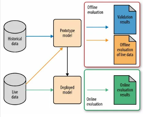
prototyping, where we try out different models to find the best one (model selection). Once we are satisfied with a prototype model, we deploy it into production, where it will go through further testing on live data.1Figure 1-1
Figure 1-1. Machine learning model development and evaluation workflow
There is not an agreed upon terminology here, but I’ll discuss this workflow in terms of “offline evaluation” and “online evaluation.” Online evaluation
measures live metrics of the deployed model on live data; offline evaluation
measures offline metrics of the prototyped model on historical data (and sometimes on live data as well).
In other words, it’s complicated. As we can see, there are a lot of colors and boxes and arrows in Figure 1-1.
different metrics, but that’s an even finer point (see the note in Chapter 2). Online evaluation, on the other hand, might measure business metrics such as customer lifetime value, which may not be available on historical data but are closer to what your business really cares about (more about picking the right metric for online evaluation in Chapter 5).
Secondly, note that there are two sources of data: historical and live. Many statistical models assume that the distribution of data stays the same over time. (The technical term is that the distribution is stationary.) But in practice, the distribution of data changes over time, sometimes drastically. This is called distribution drift. As an example, think about building a recommender for news articles. The trending topics change every day,
sometimes every hour; what was popular yesterday may no longer be relevant today. One can imagine the distribution of user preference for news articles changing rapidly over time. Hence it’s important to be able to detect
distribution drift and adapt the model accordingly.
One way to detect distribution drift is to continue to track the model’s performance on the validation metric on live data. If the performance is comparable to the validation results when the model was built, then the model still fits the data. When performance starts to degrade, then it’s probable that the distribution of live data has drifted sufficiently from
Evaluation Metrics
Chapter 2 focuses on evaluation metrics. Different machine learning tasks have different performance metrics. If I build a classifier to detect spam emails versus normal emails, then I can use classification performance
Offline Evaluation Mechanisms
As alluded to earlier, the main task during the prototyping phase is to select the right model to fit the data. The model must be evaluated on a dataset that’s statistically independent from the one it was trained on. Why? Because its performance on the training set is an overly optimistic estimate of its true performance on new data. The process of training the model has already adapted to the training data. A more fair evaluation would measure the model’s performance on data that it hasn’t yet seen. In statistical terms, this gives an estimate of the generalization error, which measures how well the model generalizes to new data.
So where does one obtain new data? Most of the time, we have just the one dataset we started out with. The statistician’s solution to this problem is to chop it up or resample it and pretend that we have new data.
Hyperparameter Search
You may have heard of terms like hyperparameter search, auto-tuning (which is just a shorter way of saying hyperparameter search), or grid search (a
possible method for hyperparameter search). Where do those terms fit in? To understand hyperparameter search, we have to talk about the difference
between a model parameter and a hyperparameter. In brief, model parameters are the knobs that the training algorithm knows how to tweak; they are
learned from data. Hyperparameters, on the other hand, are not learned by the training method, but they also need to be tuned. To make this more concrete, say we are building a linear classifier to differentiate between spam and nonspam emails. This means that we are looking for a line in feature space that separates spam from nonspam. The training process determines where that line lies, but it won’t tell us how many features (or words) to use to represent the emails. The line is the model parameter, and the number of features is the hyperparameter.
Hyperparameters can get complicated quickly. Much of the prototyping phase involves iterating between trying out different models,
hyperparameters, and features. Searching for the optimal hyperparameter can be a laborious task. This is where search algorithms such as grid search, random search, or smart search come in. These are all search methods that look through hyperparameter space and find good configurations.
Online Testing Mechanisms
Once a satisfactory model is found during the prototyping phase, it can be deployed to production, where it will interact with real users and live data. The online phase has its own testing procedure. The most commonly used form of online testing is A/B testing, which is based on statistical hypothesis testing. The basic concepts may be well known, but there are many pitfalls and challenges in doing it correctly. Chapter 5 goes into a checklist of questions to ask when running an A/B test, so as to avoid some of the pernicious pitfalls.
A less well-known form of online model selection is an algorithm called multiarmed bandits. We’ll take a look at what it is and why it might be a better alternative to A/B tests in some situations.
Without further ado, let’s get started!
1 For the sake of simplicity, we focus on “batch training” and deployment in
Chapter 2. Evaluation Metrics
Classification Metrics
Classification is about predicting class labels given input data. In binary classification, there are two possible output classes. In multiclass
classification, there are more than two possible classes. I’ll focus on binary
classification here. But all of the metrics can be extended to the multiclass scenario.
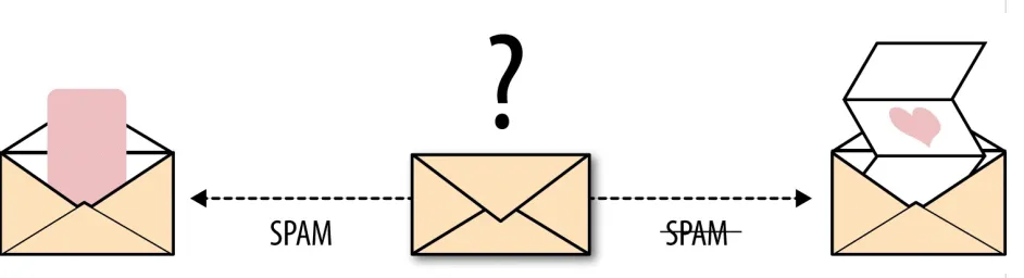
An example of binary classification is spam detection, where the input data could include the email text and metadata (sender, sending time), and the output label is either “spam” or “not spam.” (See Figure 2-1.) Sometimes, people use generic names for the two classes: “positive” and “negative,” or “class 1” and “class 0.”
There are many ways of measuring classification performance. Accuracy, confusion matrix, log-loss, and AUC are some of the most popular metrics. Precision-recall is also widely used; I’ll explain it in “Ranking Metrics”.
Accuracy
Confusion Matrix
Accuracy looks easy enough. However, it makes no distinction between classes; correct answers for class 0 and class 1 are treated equally—
sometimes this is not enough. One might want to look at how many examples failed for class 0 versus class 1, because the cost of misclassification might differ for the two classes, or one might have a lot more test data of one class than the other. For example, when a doctor makes a medical diagnosis that a patient has cancer when he doesn’t (known as a false positive) has very
different consequences than making the call that a patient doesn’t have cancer when he does (a false negative). A confusion matrix (or confusion table) shows a more detailed breakdown of correct and incorrect classifications for each class. The rows of the matrix correspond to ground truth labels, and the columns represent the prediction.
Suppose the test dataset contains 100 examples in the positive class and 200 examples in the negative class; then, the confusion table might look
something like this:
Predicted as positive Predicted as negative
Labeled as positive 80 20
Labeled as negative 5 195
Per-Class Accuracy
A variation of accuracy is the average per-class accuracy—the average of the accuracy for each class. Accuracy is an example of what’s known as a micro-average, and average per-class accuracy is a macro-average. In the above example, the average per-class accuracy would be (80% + 97.5%)/2 = 88.75%. Note that in this case, the average per-class accuracy is quite different from the accuracy.
In general, when there are different numbers of examples per class, the average per-class accuracy will be different from the accuracy. (Exercise for the curious reader: Try proving this mathematically!) Why is this important? When the classes are imbalanced, i.e., there are a lot more examples of one class than the other, then the accuracy will give a very distorted picture,
because the class with more examples will dominate the statistic. In that case, you should look at the per-class accuracy, both the average and the individual per-class accuracy numbers.
Log-Loss
Log-loss, or logarithmic loss, gets into the finer details of a classifier. In particular, if the raw output of the classifier is a numeric probability instead of a class label of 0 or 1, then log-loss can be used. The probability can be understood as a gauge of confidence. If the true label is 0 but the classifier thinks it belongs to class 1 with probability 0.51, then even though the
classifier would be making a mistake, it’s a near miss because the probability is very close to the decision boundary of 0.5. Log-loss is a “soft”
measurement of accuracy that incorporates this idea of probabilistic confidence.
Mathematically, log-loss for a binary classifier looks like this:
Formulas like this are incomprehensible without years of grueling, inhuman training. Let’s unpack it. pi is the probability that the ith data point belongs to class 1, as judged by the classifier. yi is the true label and is either 0 or 1. Since yi is either 0 or 1, the formula essentially “selects” either the left or the right summand. The minimum is 0, which happens when the prediction and the true label match up. (We follow the convention that defines 0 log 0 = 0.) The beautiful thing about this definition is that it is intimately tied to
AUC
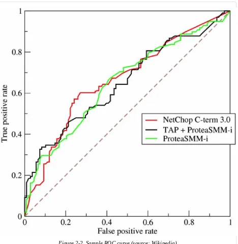
AUC stands for area under the curve. Here, the curve is the receiver operating characteristic curve, or ROC curve for short. This exotic sounding name
originated in the 1950s from radio signal analysis, and was made popular by a 1978 paper by Charles Metz called "Basic Principles of ROC Analysis.” The ROC curve shows the sensitivity of the classifier by plotting the rate of true positives to the rate of false positives (see Figure 2-2). In other words, it shows you how many correct positive classifications can be gained as you allow for more and more false positives. The perfect classifier that makes no mistakes would hit a true positive rate of 100% immediately, without
Figure 2-2. Sample ROC curve (source: Wikipedia)
automatically. A good ROC curve has a lot of space under it (because the true positive rate shoots up to 100% very quickly). A bad ROC curve covers very little area. So high AUC is good, and low AUC is not so good.
For more explanations about ROC and AUC, see this excellent tutorial by Kevin Markham. Outside of the machine learning and data science
Ranking Metrics
We’ve arrived at ranking metrics. But wait! We are not quite out of the
classification woods yet. One of the primary ranking metrics, precision-recall, is also popular for classification tasks.
Ranking is related to binary classification. Let’s look at Internet search, for example. The search engine acts as a ranker. When the user types in a query, the search engine returns a ranked list of web pages that it considers to be relevant to the query. Conceptually, one can think of the task of ranking as first a binary classification of “relevant to the query” versus “irrelevant to the query,” followed by ordering the results so that the most relevant items
appear at the top of the list. In an underlying implementation, the classifier may assign a numeric score to each item instead of a categorical class label, and the ranker may simply order the items by the raw score.
Precision-Recall
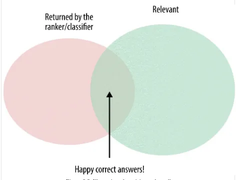
Precision and recall are actually two metrics. But they are often used together. Precision answers the question, “Out of the items that the ranker/classifier predicted to be relevant, how many are truly relevant?” Whereas, recall answers the question, “Out of all the items that are truly relevant, how many are found by the ranker/classifier?” Figure 2-3 contains a simple Venn diagram that illustrates precision versus recall.
Figure 2-3. Illustration of precision and recall
Frequently, one might look at only the top k items from the ranker, k = 5, 10, 20, 100, etc. Then the metrics would be called “precision@k” and
“recall@k.”
When dealing with a recommender, there are multiple “queries” of interest; each user is a query into the pool of items. In this case, we can average the precision and recall scores for each query and look at “average precision@k” and “average recall@k.” (This is analogous to the relationship between
Precision-Recall Curve and the F1 Score
When we change k, the number of answers returned by the ranker, the precision and recall scores also change. By plotting precision versus recall over a range of k values, we get the precision-recall curve. This is closely related to the ROC curve. (Exercise for the curious reader: What’s the relationship between precision and the false-positive rate? What about recall?)
Just like it’s difficult to compare ROC curves to each other, the same goes for the precision-recall curve. One way of summarizing the precision-recall curve is to fix k and combine precision and recall. One way of combining these two numbers is via their harmonic mean:
NDCG
Precision and recall treat all retrieved items equally; a relevant item in
position k counts just as much as a relevant item in position 1. But this is not usually how people think. When we look at the results from a search engine, the top few answers matter much more than answers that are lower down on the list.
NDCG tries to take this behavior into account. NDCG stands for normalized discounted cumulative gain. There are three closely related metrics here: cumulative gain (CG), discounted cumulative gain (DCG), and finally, normalized discounted cumulative gain. Cumulative gain sums up the
relevance of the top k items. Discounted cumulative gain discounts items that are further down the list. Normalized discounted cumulative gain, true to its name, is a normalized version of discounted cumulative gain. It divides the DCG by the perfect DCG score, so that the normalized score always lies between 0.0 and 1.0. See the Wikipedia article for detailed mathematical formulas.
Regression Metrics
RMSE
The most commonly used metric for regression tasks is RMSE (root-mean-square error), also known as RMSD (root-mean-(root-mean-square deviation). This is defined as the square root of the average squared distance between the actual score and the predicted score:
Here, yi denotes the true score for the ith data point, and denotes the
Quantiles of Errors
RMSE may be the most common metric, but it has some problems. Most crucially, because it is an average, it is sensitive to large outliers. If the
regressor performs really badly on a single data point, the average error could be very big. In statistical terms, we say that the mean is not robust (to large outliers).
Quantiles (or percentiles), on the other hand, are much more robust. To see why this is, let’s take a look at the median (the 50th percentile), which is the element of a set that is larger than half of the set, and smaller than the other half. If the largest element of a set changes from 1 to 100, the mean should shift, but the median would not be affected at all.
One thing that is certain with real data is that there will always be “outliers.” The model will probably not perform very well on them. So it’s important to look at robust estimators of performance that aren’t affected by large outliers. It is useful to look at the median absolute percentage:
“Almost Correct” Predictions
Caution: The Difference Between Training
Metrics and Evaluation Metrics
Sometimes, the model training procedure may use a different metric (also known as a loss function) than the evaluation. This can happen when we are reappropriating a model for a different task than it was designed for. For instance, we might train a personalized recommender by minimizing the loss between its predictions and observed ratings, and then use this recommender to produce a ranked list of recommendations.
This is not an optimal scenario. It makes the life of the model difficult—it’s being asked to do a task that it was not trained to do! Avoid this when
Caution: Skewed Datasets—Imbalanced
Classes, Outliers, and Rare Data
It’s easy to write down the formula of a metric. It’s not so easy to interpret the actual metric measured on real data. Book knowledge is no substitute for working experience. Both are necessary for successful applications of
machine learning.
Always think about what the data looks like and how it affects the metric. In particular, always be on the look out for data skew. By data skew, I mean the situations where one “kind” of data is much more rare than others, or when there are very large or very small outliers that could drastically change the metric.
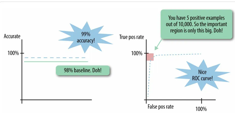
Earlier, we mentioned how imbalanced classes could be a caveat in
measuring per-class accuracy. This is one example of data skew—one of the classes is much more rare compared to the other class. It is problematic not just for per-class accuracy, but for all of the metrics that give equal weight to each data point. Suppose the positive class is only a tiny portion of the
Figure 2-4. Illustration of classification accuracy and AUC under imbalanced classes
Any metric that gives equal weight to each instance of a class has a hard time handling imbalanced classes, because by definition, the metric will be
dominated by the class(es) with the most data. Furthermore, they are
problematic not only for the evaluation stage, but even more so when training the model. If class imbalance is not properly dealt with, the resulting model may not know how to predict the rare classes at all.
Data skew can also create problems for personalized recommenders. Real-world user-item interaction data often contains many users who rate very few items, as well as items that are rated by very few users. Rare users and rare items are problematic for the recommender, both during training and
evaluation. When not enough data is available in the training data, a
recommender model would not be able to learn the user’s preferences, or the items that are similar to a rare item. Rare users and items in the evaluation data would lead to a very low estimate of the recommender’s performance, which compounds the problem of having a badly trained recommender.
Related Reading
An Introduction to ROC Analysis”.Tom Fawcett. Pattern Recognition Letters, 2006.
Software Packages
Many of the metrics (and more) are implemented in various software packages for data science.
R: Metrics package.
Chapter 3. Offline Evaluation
Mechanisms: Hold-Out
Validation, Cross-Validation,
and Bootstrapping
Unpacking the Prototyping Phase: Training,
Validation, Model Selection
Each time we tweak something, we come up with a new model. Model
selection refers to the process of selecting the right model (or type of model) that fits the data. This is done using validation results, not training results.
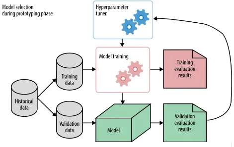
Figure 3-1. The prototyping phase of building a machine learning model
In Figure 3-1, hyperparameter tuning is illustrated as a “meta” process that controls the training process. We’ll discuss exactly how it is done in
Chapter 4. Take note that the available historical dataset is split into two parts: training and validation. The model training process receives training data and produces a model, which is evaluated on validation data. The results from validation are passed back to the hyperparameter tuner, which tweaks some knobs and trains the model again.
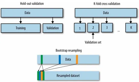
In the offline setting, all we have is one historical dataset. Where might we obtain another independent set? We need a testing mechanism that generates additional datasets. We can either hold out part of the data, or use a
resampling technique such as cross-validation or bootstrapping. Figure 3-2
illustrates the difference between the three validation mechanisms.
Why Not Just Collect More Data?
Cross-validation and bootstrapping were invented in the age of “small data.” Prior to the age of Big Data, data collection was difficult and statistical studies were conducted on very small datasets. In 1908, the statistician William Sealy Gosset published the Student’s t-distribution on a whopping 3000 records—tiny by today’s standards but impressive back then. In 1967, the social psychologist Stanley Milgram and associates ran the famous small world experiment on a total of 456 individuals, thereby establishing the notion of “six degrees of separation” between any two persons in a social network. Another study of social networks in the 1960s involved solely 18 monks living in a monastery. How can one manage to come up with any statistically convincing conclusions given so little data?
One has to be clever and frugal with data. The cross-validation, jackknife, and bootstrap mechanisms resample the data to produce multiple datasets. Based on these, one can calculate not just an average estimate of test
Hold-Out Validation
Hold-out validation is simple. Assuming that all data points are i.i.d.
(independently and identically distributed), we simply randomly hold out part of the data for validation. We train the model on the larger portion of the data and evaluate validation metrics on the smaller hold-out set.
Computationally speaking, hold-out validation is simple to program and fast to run. The downside is that it is less powerful statistically. The validation results are derived from a small subset of the data, hence its estimate of the generalization error is less reliable. It is also difficult to compute any variance information or confidence intervals on a single dataset.
Cross-Validation
Cross-validation is another validation technique. It is not the only validation technique, and it is not the same as hyperparameter tuning. So be careful not to get the three (the concept of model validation, cross-validation, and
hyperparameter tuning) confused with each other. Cross-validation is simply a way of generating training and validation sets for the process of
hyperparameter tuning. Hold-out validation, another validation technique, is also valid for hyperparameter tuning, and is in fact computationally much cheaper.
There are many variants of cross-validation. The most commonly used is k-fold cross-validation. In this procedure, we first divide the training dataset into k folds (see Figure 3-2). For a given hyperparameter setting, each of the k folds takes turns being the hold-out validation set; a model is trained on the rest of the k – 1 folds and measured on the held-out fold. The overall
performance is taken to be the average of the performance on all k folds. Repeat this procedure for all of the hyperparameter settings that need to be evaluated, then pick the hyperparameters that resulted in the highest k-fold average.
Another variant of cross-validation is leave-one-out cross-validation. This is essentially the same as k-fold cross-validation, where k is equal to the total number of data points in the dataset.
Bootstrap and Jackknife
Bootstrap is a resampling technique. It generates multiple datasets by sampling from a single, original dataset. Each of the “new” datasets can be used to estimate a quantity of interest. Since there are multiple datasets and therefore multiple estimates, one can also calculate things like the variance or a confidence interval for the estimate.
Bootstrap is closely related to cross-validation. It was inspired by another resampling technique called the jackknife, which is essentially leave-one-out cross-validation. One can think of the act of dividing the data into k folds as a (very rigid) way of resampling the data without replacement; i.e., once a data point is selected for one fold, it cannot be selected again for another fold. Bootstrap, on the other hand, resamples the data with replacement. Given a dataset containing N data points, bootstrap picks a data point uniformly at random, adds it to the bootstrapped set, puts that data point back into the dataset, and repeats.
Why put the data point back? A real sample would be drawn from the real distribution of the data. But we don’t have the real distribution of the data. All we have is one dataset that is supposed to represent the underlying distribution. This gives us an empirical distribution of data. Bootstrap
simulates new samples by drawing from the empirical distribution. The data point must be put back, because otherwise the empirical distribution would change after each draw.
Obviously, the bootstrapped set may contain the same data point multiple times. (See Figure 3-2 for an illustration.) If the random draw is repeated N times, then the expected ratio of unique instances in the bootstrapped set is approximately 1 – 1/e ≈ 63.2%. In other words, roughly two-thirds of the original dataset is expected to end up in the bootstrapped dataset, with some amount of replication.
Caution: The Difference Between Model
Validation and Testing
Thus far I’ve been careful to avoid the word “testing.” This is because model validation is a different step than model testing. This is a subtle point. So let me take a moment to explain it.
The prototyping phase revolves around model selection, which requires measuring the performance of one or more candidate models on one or more validation datasets. When we are satisfied with the selected model type and hyperparameters, the last step of the prototyping phase should be to train a new model on the entire set of available data using the best hyperparameters found. This should include any data that was previously held aside for
validation. This is the final model that should be deployed to production. Testing happens after the prototyping phase is over, either online in the production system or offline as a way of monitoring distribution drift, as discussed earlier in this chapter.
Never mix training data and evaluation data. Training, validation, and testing should happen on different datasets. If information from the validation data or test data leaks into the training procedure, it would lead to a bad estimate of generalization error, which then leads to bitter tears of regret.
Summary
To recap, here are the important points for offline evaluation and model validation:
1. During the model prototyping phase, one needs to do model selection. This involves hyperparameter tuning as well as model training. Every new model needs to be evaluated on a separate dataset. This is called model validation.
2. validation is not the same as hyperparameter tuning. Cross-validation is a mechanism for generating training and Cross-validation splits. Hyperparameter tuning is the mechanism by which we select the best hyperparameters for a model; it might use cross-validation to evaluate the model.
3. Hold-out validation is an alternative to cross-validation. It is simpler testing and computationally cheaper. I recommend using hold-out validation as long as there is enough data to be held out.
4. Cross-validation is useful when the dataset is small, or if you are extra paranoid.
Related Reading
Software Packages
R: cvTools
Chapter 4. Hyperparameter
Tuning
Model Parameters Versus Hyperparameters
First, let’s define what a hyperparameter is, and how it is different from a normal nonhyper model parameter.
Machine learning models are basically mathematical functions that represent the relationship between different aspects of data. For instance, a linear regression model uses a line to represent the relationship between “features” and “target.” The formula looks like this:
where x is a vector that represents features of the data and y is a scalar variable that represents the target (some numeric quantity that we wish to learn to predict).
This model assumes that the relationship between x and y is linear. The variable w is a weight vector that represents the normal vector for the line; it specifies the slope of the line. This is what’s known as a model parameter, which is learned during the training phase. “Training a model” involves using an optimization procedure to determine the best model parameter that “fits” the data.
There is another set of parameters known as hyperparameters, sometimes also knowns as “nuisance parameters.” These are values that must be
specified outside of the training procedure. Vanilla linear regression doesn’t have any hyperparameters. But variants of linear regression do. Ridge
regression and lasso both add a regularization term to linear regression; the weight for the regularization term is called the regularization parameter. Decision trees have hyperparameters such as the desired depth and number of leaves in the tree. Support vector machines (SVMs) require setting a
What Do Hyperparameters Do?
A regularization hyperparameter controls the capacity of the model, i.e., how flexible the model is, how many degrees of freedom it has in fitting the data. Proper control of model capacity can prevent overfitting, which happens when the model is too flexible, and the training process adapts too much to the training data, thereby losing predictive accuracy on new test data. So a proper setting of the hyperparameters is important.
Another type of hyperparameter comes from the training process itself. Training a machine learning model often involves optimizing a loss function (the training metric). A number of mathematical optimization techniques may be employed, some of them having parameters of their own. For instance, stochastic gradient descent optimization requires a learning rate or a learning schedule. Some optimization methods require a convergence threshold.
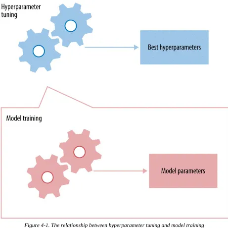
Hyperparameter Tuning Mechanism
Hyperparameter settings could have a big impact on the prediction accuracy of the trained model. Optimal hyperparameter settings often differ for
different datasets. Therefore they should be tuned for each dataset. Since the training process doesn’t set the hyperparameters, there needs to be a meta process that tunes the hyperparameters. This is what we mean by
hyperparameter tuning.
Figure 4-1. The relationship between hyperparameter tuning and model training
Example 4-1. Pseudo-Python code for a very simple hyperparameter tuner func hyperparameter_tuner (training_data,
validation_data, hp_list):
hp_perf = []
# train and evaluate on all hyperparameter settings
foreach hp_setting in hp_list:
m = train_model(training_data, hp_setting)
validation_results = eval_model(m, validation_data) hp_perf.append(validation_results)
# find the best hyperparameter setting
best_hp_setting = hp_list[max_index(hp_perf)]
# IMPORTANT:
# train a model on *all* available data using the best
# hyperparameters
best_m = train_model(training_data.append(validation_data), best_hp_setting)
return (best_hp_setting, best_m)
Hyperparameter Tuning Algorithms
Conceptually, hyperparameter tuning is an optimization task, just like model training.
However, these two tasks are quite different in practice. When training a model, the quality of a proposed set of model parameters can be written as a mathematical formula (usually called the loss function). When tuning
hyperparameters, however, the quality of those hyperparameters cannot be written down in a closed-form formula, because it depends on the outcome of a black box (the model training process).
Grid Search
Grid search, true to its name, picks out a grid of hyperparameter values, evaluates every one of them, and returns the winner. For example, if the hyperparameter is the number of leaves in a decision tree, then the grid could be 10, 20, 30, …, 100. For regularization parameters, it’s common to use exponential scale: 1e-5, 1e-4, 1e-3, …, 1. Some guesswork is necessary to specify the minimum and maximum values. So sometimes people run a small grid, see if the optimum lies at either endpoint, and then expand the grid in that direction. This is called manual grid search.
Random Search
I love movies where the underdog wins, and I love machine learning papers where simple solutions are shown to be surprisingly effective. This is the storyline of “Random Search for Hyper Parameter Optimization” by Bergstra and Bengio. Random search is a slight variation on grid search. Instead of searching over the entire grid, random search only evaluates a random sample of points on the grid. This makes random search a lot cheaper than grid
search. Random search wasn’t taken very seriously before. This is because it doesn’t search over all the grid points, so it cannot possibly beat the optimum found by grid search. But then along came Bergstra and Bengio. They
showed that, in surprisingly many instances, random search performs about as well as grid search. All in all, trying 60 random points sampled from the grid seems to be good enough.
In hindsight, there is a simple probabilistic explanation for the result: for any distribution over a sample space with a finite maximum, the maximum of 60 random observations lies within the top 5% of the true maximum, with 95% probability. That may sound complicated, but it’s not. Imagine the 5%
interval around the true maximum. Now imagine that we sample points from this space and see if any of them land within that maximum. Each random draw has a 5% chance of landing in that interval; if we draw n points
independently, then the probability that all of them miss the desired interval is (1 – 0.05)n. So the probability that at least one of them succeeds in hitting
the interval is 1 minus that quantity. We want at least a 0.95 probability of success. To figure out the number of draws we need, just solve for n in the following equation:
1 – (1 – 0.05)n > 0.95
We get n >= 60. Ta-da!
there is a high concentration of grid points in that region. The former is more likely, because a good machine learning model should not be overly sensitive to the hyperparameters, i.e., the close-to-optimal region is large.
With its utter simplicity and surprisingly reasonable performance, random search is my go-to method for hyperparameter tuning. It’s trivially
Smart Hyperparameter Tuning
Smarter tuning methods are available. Unlike the “dumb” alternatives of grid search and random search, smart hyperparameter tuning is much less
parallelizable. Instead of generating all the candidate points up front and evaluating the batch in parallel, smart tuning techniques pick a few
hyperparameter settings, evaluate their quality, then decide where to sample next. This is an inherently iterative and sequential process. It is not very parallelizable. The goal is to make fewer evaluations overall and save on the overall computation time. If wall clock time is your goal, and you can afford multiple machines, then I suggest sticking to random search.
Buyer beware: smart search algorithms require computation time to figure out where to place the next set of samples. Some algorithms require much more time than others. Hence it only makes sense if the evaluation procedure—the inner optimization box—takes much longer than the process of evaluating where to sample next. Smart search algorithms also contain parameters of their own that need to be tuned. (Hyper-hyperparameters?) Sometimes tuning the hyper-hyperparameters is crucial to make the smart search algorithm faster than random search.
Recall that hyperparameter tuning is difficult because we cannot write down the actual mathematical formula for the function we’re optimizing. (The technical term for the function that is being optimized is response surface.) Consequently, we don’t have the derivative of that function, and therefore most of the mathematical optimization tools that we know and love, such as the Newton method or stochastic gradient descent (SGD), cannot be applied. I will highlight three smart tuning methods proposed in recent years:
derivative-free optimization, Bayesian optimization, and random forest smart tuning. Derivative-free methods employ heuristics to determine where to sample next. Bayesian optimization and random forest smart tuning both model the response surface with another function, then sample more points based on what the model says.
to model the response function and something called Expected Improvement to determine the next proposals. Gaussian processes are trippy; they specify distributions over functions. When one samples from a Gaussian process, one generates an entire function. Training a Gaussian process adapts this
distribution over the data at hand, so that it generates functions that are more likely to model all of the data at once. Given the current estimate of the
function, one can compute the amount of expected improvement of any point over the current optimum. They showed that this procedure of modeling the hyperparameter response surface and generating the next set of proposed hyperparameter settings can beat the evaluation cost of manual tuning.
Frank Hutter, Holger H. Hoos, and Kevin Leyton-Brown suggested training a random forest of regression trees to approximate the response surface. New points are sampled based on where the random forest considers to be the optimal regions. They call this SMAC (Sequential Model-based Algorithm Configuration). Word on the street is that this method works better than Gaussian processes for categorical hyperparameters.
Derivative-free optimization, as the name suggests, is a branch of mathematical optimization for situations where there is no derivative
information. Notable derivative-free methods include genetic algorithms and the Nelder-Mead method. Essentially, the algorithms boil down to the
following: try a bunch of random points, approximate the gradient, find the most likely search direction, and go there. A few years ago, Misha Bilenko and I tried Nelder-Mead for hyperparameter tuning. We found the algorithm delightfully easy to implement and no less efficient that Bayesian
The Case for Nested Cross-Validation
Before concluding this chapter, we need to go up one more level and talk about nested cross-validation, or nested hyperparameter tuning. (I suppose this makes it a meta-meta-learning task.)
There is a subtle difference between model selection and hyperparameter tuning. Model selection can include not just tuning the hyperparameters for a particular family of models (e.g., the depth of a decision tree); it can also include choosing between different model families (e.g., should I use decision tree or linear SVM?). Some advanced hyperparameter tuning methods claim to be able to choose between different model families. But most of the time this is not advisable. The hyperparameters for different kinds of models have nothing to do with each other, so it’s best not to lump them together.
Choosing between different model families adds one more layer to our cake of prototyping models. Remember our discussion about why one must never mix training data and evaluation data? This means that we now must set aside validation data (or do cross-validation) for the hyperparameter tuner.
To make this precise, Example 4-2 shows the pseudocode in Python form. I use hold-out validation because it’s simpler to code. You can do cross-validation or bootstrap cross-validation, too. Note that at the end of each for loop, you should train the best model on all the available data at this stage.
Example 4-2. Pseudo-Python code for nested hyperparameter tuning func nested_hp_tuning(data, model_family_list):
perf_list = [] hp_list = []
for mf in model_family_list:
# generate_hp_candidates should be a function that knows
# how to generate candidate hyperparameter settings
# for any given model family
hp_settings_list = generate_hp_candidates(mf)
# run hyperparameter tuner to find best hyperparameters
# find best model family (max_index is a helper function
# that finds the index of the maximum element in a list)
best_mf = model_family_list[max_index(perf_list)] best_hp = hp_list[max_index(perf_list)]
# train a model from the best model family using all of
# the data
model = train_mf_model(best_mf, best_hp, data) return (best_mf, best_hp, model)
Related Reading
“Random Search for Hyper-Parameter Optimization.” James Bergstra and Yoshua Bengio. Journal of Machine Learning Research, 2012.
“Algorithms for Hyper-Parameter Optimization.” James Bergstra, Rémi Bardenet, Yoshua Bengio, and Balázs Kégl.” Neural Information
Processing Systems, 2011. See also a SciPy 2013 talk by the authors.
“Practical Bayesian Optimization of Machine Learning Algorithms.”
Jasper Snoek, Hugo Larochelle, and Ryan P. Adams. Neural Information Processing Systems, 2012.
“Sequential Model-Based Optimization for General Algorithm
Configuration.” Frank Hutter, Holger H. Hoos, and Kevin Leyton-Brown.
Learning and Intelligent Optimization, 2011.
“Lazy Paired Hyper-Parameter Tuning.” Alice Zheng and Mikhail
Bilenko. International Joint Conference on Artificial Intelligence, 2013.
Introduction to Derivative-Free Optimization (MPS-SIAM Series on
Optimization). Andrew R. Conn, Katya Scheinberg, and Luis N. Vincente, 2009.
Gradient-Based Hyperparameter Optimization Through Reversible Learning. Dougal Maclaurin, David Duvenaud, and Ryan P. Adams.
Software Packages
Grid search and random search: GraphLab Create, scikit-learn.
Bayesian optimization using Gaussian processes: Spearmint (from Jasper et al.)
Bayesian optimization using Tree-based Parzen Estimators: Hyperopt
(from Bergstra et al.)
Random forest tuning: SMAC (from Hutter et al.)
Chapter 5. The Pitfalls of A/B
Testing
Figure 5-1. (Source: Eric Wolfe | Dato Design)
Thus far in this report, I’ve mainly focused on introducing the basic concepts in evaluating machine learning, with an occasional cautionary note here and there. This chapter is just the opposite. I’ll give a cursory overview of the basics of A/B testing, and focus mostly on best practice tips. This is because there are many books and articles that teach statistical hypothesis testing, but relatively few articles about what can go wrong.
A/B testing is a widespread practice today. But a lot can go wrong in setting it up and interpreting the results. We’ll discuss important questions to
Recall that there are roughly two regimes for machine learning evaluation: offline and online. Offline evaluation happens during the prototyping phase where one tries out different features, models, and hyperparameters. It’s an iterative process of many rounds of evaluation against a chosen baseline on a set of chosen evaluation metrics. Once you have a model that performs
reasonably well, the next step is to deploy the model to production and evaluate its performance online, i.e., on live data. This chapter discusses
A/B Testing: What Is It?
A/B testing has emerged as the predominant method of online testing in the industry today. It is often used to answer questions like, “Is my new model better than the old one?” or “Which color is better for this button, yellow or blue?” In the A/B testing setup, there is a new model (or design) and an incumbent model (or design). There is some notion of live traffic, which is split into two groups: A and B, or control and experiment. Group A is routed to the old model, and group B is routed to the new model. Their performance is compared and a decision is made about whether the new model performs substantially better than the old model. That is the rough idea, and there is a whole statistical machinery that makes this statement much more precise. This machinery is known as statistical hypothesis testing. It decides between a null hypothesis and an alternate hypothesis. Most of the time, A/B tests are formulated to answer the question, “Does this new model lead to a
statistically significant change in the key metric?” The null hypothesis is often “the new model doesn’t change the average value of the key metric,” and the alternative hypothesis “the new model changes the average value of the key metric.” The test for the average value (the population mean, in statistical speak) is the most common, but there are tests for other population parameters as well.
There are many books and online resources that describe statistical
hypothesis testing in rigorous detail. I won’t attempt to replicate them here. For the uninitiated, www.evanmiller.org/ provides an excellent starting point that explains the details of hypothesis testing and provides handy software utilities.
Briefly, A/B testing involves the following steps:
1. Split into randomized control/experimentation groups.
2. Observe behavior of both groups on the proposed methods.
4. Compute p-value.
5. Output decision.
Simple enough. What could go wrong?
1. Complete Separation of Experiences
First, take a look at your user randomization and group splitting module. Does it cleanly split off a portion of your users for the experimentation group? Are they experiencing only the new design (or model, or whatever)? It’s important to cleanly and completely separate the experiences between the two groups. Suppose you are testing a new button for your website. If the button appears on every page, then make sure the same user sees the same button everywhere. It’ll be better to split by user ID (if available) or user sessions instead of individual page visits.
Also watch out for the possibility that some of your users have been
permanently “trained” by the old model or design and prefer the way things were before. In their KDD 2012 paper, Kohavi et al. calls this the carryover effect. Such users carry the “baggage of the old” and may return biased answers for any new model. If you think this might be the case, think about acquiring a brand new set of users or randomizing the test buckets.
It’s always good to do some A/A testing to make sure that your testing
framework is sound. In other words, perform the randomization and the split, but test both groups on the same model or design. See if there are any
2. Which Metric?
The next important question is, on which metric should you evaluate the model? Ultimately, the right metric is probably a business metric. But this may not be easily measurable in the system. For instance, search engines care about the number of users, how long they spend on the site, and their overall market share. Comparison statistics are not readily available to the live system. So they will need to approximate the ultimate business metric of market share with measurable ones like number of unique visitors per day and average session length. In practice, short-term, measurable live metrics may not always align with long-term business metrics, and it can be tricky to design the right metric.
Backing up for a second, there are four classes of metrics to think about: business metrics, measurable live metrics, offline evaluation metrics, and training metrics. We just discussed the difference between business metrics and live metrics that can be measured. Offline evaluation metrics are things like the classification, regression, and ranking metrics we discussed
previously. The training metric is the loss function that is optimized during the training process. (For example, a support vector machine optimizes a combination of the norm of the weight vector and misclassification
penalties.)
3. How Much Change Counts as Real Change?
4. One-Sided or Two-Sided Test?
5. How Many False Positives Are You Willing to
Tolerate?
A false positive in A/B testing means that you’ve rejected the null hypothesis when the null hypothesis is true. In other words, you’ve decided that your model is better than the baseline when it isn’t better than the baseline. What’s the cost of a false positive? The answer depends on the application.
In a drug effectiveness study, a false positive could cause the patient to use an ineffective drug. Conversely, a false negative could mean not using a drug that is effective at curing the disease. Both cases could have a very high cost to the patient’s health.
In a machine learning A/B test, a false positive might mean switching to a model that should increase revenue when it doesn’t. A false negative means missing out on a more beneficial model and losing out on potential revenue increase.
6. How Many Observations Do You Need?
The number of observations is partially determined by the desired statistical power. This must be determined prior to running the test. A common
temptation is to run the test until you observe a significant result. This is wrong.
The power of a test is its ability to correctly identify the positives, e.g.,
correctly determine that a new model is doing well when it is in fact superior. It can be written as a formula that involves the significance level (question #5), the difference between the control and experimentation metrics (question #3), and the size of the samples (the number of observations included in the control and the experimentation group). You pick the right value for power, significance level, and the desired amount of change. Then you can compute how many observations you need in each group. A recent blog post from
StitchFix goes through the power analysis in minute detail.
As explained in detail on Evan Miller’s website, do NOT stop the test until you’ve accumulated this many observations! Specifically, do not stop the test as soon as you detect a “significant” difference. The answer is not to be
7. Is the Distribution of the Metric Gaussian?
The vast majority of A/B tests use the t-test. But the t-test makes assumptions that are not always satisfied by all metrics. It’s a good idea to look at the distribution of your metric and check whether the assumptions of the t-test are valid.
The t-test assumes that the two populations are Gaussian distributed. Does your metric fit a Gaussian distribution? The common hand-wavy justification is to say, “Almost everything converges to a Gaussian distribution due to the Central Limit Theorem.” This is usually true when:
1. The metric is an average.
2. The distribution of metric values has one mode.
3. The metric is distributed symmetrically around this mode.
These are actually easily violated in real-world situations. For example, the accuracy or the click-through rate is an average, but the area under the curve (AUC) is not. (It is an integral.) The distribution of the metric may not have one mode if there are multiple user populations within the control or
experimental group. The metric is not symmetric if, say, it can be any positive number but can never be negative. Kohavi et al. gives examples of metrics that are definitely not Gaussian and whose standard error does not decrease with longer tests. For example, metrics involving counts are better modeled as negative binomials.
When these assumptions are violated, the distribution may take longer than usual to converge to a Gaussian, or not at all. Usually, the average of more than 30 observations starts to look like a Gaussian. When there is a mixture of populations, however, it will take much longer. Here are a few rules of thumb that can mitigate the violation of t-test assumptions:
2. Alternatively, the family of power transforms tends to stabilize the variance (decrease the variance or at least make it not dependent on the mean) and make the distribution more Gaussian-like.
3. The negative binomial is a better distribution for counts.
8. Are the Variances Equal?
Okay, you checked and double-checked and you’re really sure that the distribution is a Gaussian, or will soon become a Gaussian. Fine. Next
question: are the variances equal for the control and the experimental group? If the groups are split fairly (uniformly at random), the variances are probably equal. However, there could be subtle biases in your stream splitter (see
question #1). Or perhaps one population is much smaller compared to the other. Welch’s t-test is a little-known alternative to the much more common Student’s t-test. Unlike Student’s t-test, Welch’s t-test does not assume equal variance. For this reason, it is a more robust alternative. Here’s what
Wikipedia says about the advantages and limitations of Welch’s t-test:
Welch’s t-test is more robust than Student’s t-test and maintains type I error rates close to nominal for unequal variances and for unequal sample sizes. Furthermore, the power of Welch’s t-test comes close to that of
Student’s t-test, even when the population variances are equal and sample sizes are balanced.
It is not recommended to pre-test for equal variances and then choose between Student’s t-test or Welch’s t-test. Rather, Welch’s t-test can be applied directly and without any substantial disadvantages to Student’s t-test as noted above. Welch’s t-t-test remains robust for skewed distributions and large sample sizes. Reliability decreases for skewed distributions and smaller samples, where one could possibly perform Welch’s t-test on ranked data.
In practice, this may not make too big of a difference, because the
9. What Does the p-Value Mean?
As Cosma Shalizi explained in his very detailed and technical blog post, most people interpret the p-value incorrectly. A small p-value does not imply a significant result. A smaller p-value does not imply a more significant result. The p-value is a function of the size of the samples, the difference between the two populations, and how well we can estimate the true means. I’ll leave the curious, statistically minded reader to digest the blog post (highly
recommended!). The upshot is that, in addition to running the hypothesis test and computing the p-value, one should always check the confidence interval of the two population mean estimates. If the distribution is close to being Gaussian, then the usual standard error estimation applies. Otherwise, compute a bootstrap estimate, which we discussed in Chapter 3. This can differentiate between the two cases of “there is indeed a significant difference between the two populations” versus “I can’t tell whether there is a difference because the variances of the estimates are too high so I can’t trust the
10. Multiple Models, Multiple Hypotheses
So you are a hard-working data scientist and you have not one but five new models you want to test. Or maybe 328 of them. Your website has so much traffic that you have no problem splitting off a portion of the incoming traffic to test each of the models at the same time. Parallel A1/.../Am/B testing, here we come!
But wait, now you are in the situation of multiple hypothesis testing. Remember the false positive rate we talked about in question #5? Testing multiple hypotheses increases the overall false positive probability. If one test has a false positive rate of 0.05, then the probability that none of the 20 tests makes a false positive drops precipitously to (1 – 0.05)20 = 0.36. What’s
more, this calculation assumes that the tests are independent. If the tests are not independent (i.e., maybe your 32 models all came from the same training dataset?), then the probability of a false positive may be even higher.
Benjamini and Hochberg proposed a useful method for dealing with false positives in multiple tests. In their 1995 paper, “Controlling the False Discovery Rate: A Practical and Powerful Approach to Multiple Testing,” they proposed a modified procedure that orders the p-values from each test and rejects the null hypothesis for the smallest normalized p-values (
, where q is the desired significance level, m is the total number of tests, and i is the ranking of the p-value). This test does not assume that the tests are independent or are normally distributed, and has more statistical power than the classic Bonferroni correction.
Even without running multiple tests simultaneously, you may still run into the multiple hypothesis testing scenario. For instance, if you are changing your model based on live test data, submitting new models until something achieves the acceptance threshold, then you are essentially running multiple tests sequentially. It’s a good idea to apply the Benjamini-Hochberg
11. How Long to Run the Test?
The answer to how long to run your A/B test depends not just on the number of observations you need in order to achieve the desired statistical power (question #6). It also has to do with the user experience.
In some fields, such as pharmaceutical drug testing, running the test too long has ethical consequences for the user; if the drug is already proven to be effective, then stopping the trial early may save lives in the control group. Balancing the need for early stopping and sufficient statistical power led to the study of sequential analysis, where early stopping points are determined a priori at the start of the trials.
In most newly emergent machine learning applications, running the test longer is not as big of a problem. More likely, the constraint is distribution drift, where the behavior of the user changes faster than one can collect enough observations. (See question #12.)
When determining the length of a trial, it’s important to go beyond what’s known as the Novelty effect. When users are switched to a new experience, their initial reactions may not be their long-term reactions. In other words, if you are testing a new color for a button, the user may initially love the button and click it more often, just because it’s novel, or she may hate the new color and never touch it, but eventually she would get used to the new color and behave as she did before. It’s important to run the trial long enough to get past the period of the “shock of the new.”