Methodological issues in
cross-country
r
region decomposition of
energy and environment indicators
F.Q. Zhang, B.W. Ang
UDepartment of Industrial and Systems Engineering, National Uni¨ersity of Singapore, 10 Kent Ridge Crescent, Singapore 119260, Singapore
Abstract
A recent development in energy and environment decomposition analysis is the
applica-tion of the technique to cross-countryrregion comparisons. Cross-countryrregion
decompo-sition gives rise to several problems that do not normally occur in chronological decomposi-tion of changes in a specific country. These include large variadecomposi-tions in explanatory factors in the data, the measure of economic output and structural comparability. We examine these
problems using energy-related CO emission data of three world regions. It is concluded2
that the conventional decomposition methods are not effective in cross-countryrregion
studies as they tend to leave a large residual. Instead, perfect decomposition methods should be adopted. The choice of economic output measure can affect decomposition results
greatly and the impacts vary from one decomposition method to another.䊚 2001 Elsevier
Science B.V. All rights reserved.
JEL classifications:C50; Q41
Keywords:Decomposition methodology; CO emissions; Cross-country comparisons2
1. Introduction
The past two decades have seen many studies dealing with decomposition of changes in energy and environmental indicators, such as aggregate energy con-sumptionrintensity and aggregate CO emissions2 rintensity. Almost all these
stud-U
Corresponding author. Tel.:q65-8742203; fax:q65-7771434.
Ž .
E-mail address:[email protected] B.W. Ang .
0140-9883r01r$ - see front matter䊚2001 Elsevier Science B.V. All rights reserved.
Ž .
ies dealt with decomposition of changes in an aggregate over time in a specific country or region. As far as we know, only three and fairly recent studies dealt with
Ž .
decomposition across country or region. In the study by Proops et al. 1993 , cross-country decomposition of CO2 emissions in Germany and the UK was
Ž .
conducted. Chung 1998 investigated differences in energy-related CO emissions2 in industry in China, Japan and South Korea. Both studies adopted the input᎐
output structural decomposition approach. More recently, inter-region decomposi-tion of energy-related CO emissions in three world regions using the index2
Ž .
decomposition approach was reported in Ang and Zhang 1999 . The main empha-sis of these three studies is primarily empirical. Of interest to the authors are the identification of factors and the relative contributions of these factors to the differences in CO emissions between the countries or regions studied.2
Cross-country decomposition studies allow analysts and decision-makers to have a better understanding of the underlying causes of variation in an aggregate between countries. There are, however, some specific problems in cross-country decomposition that do not normally arise in decomposition of changes of an aggregate over time in a country. These problems have so far not been addressed in detail in the context of decomposition studies. Cross-country decomposition is often characterized by large variations in explanatory factors, such as GDP and fuel shares in energy consumption, which arise from inherent differences between the countries compared. In such a situation, application of the conventional decomposition methods could lead to a large residual which makes result
interpre-Ž .
tation very difficult. In the study by Chung 1998 , for instance, the residual amounts to 18% of the difference in CO emissions between China and South2
Korea. To overcome such a problem, some recently proposed perfect decomposi-tion methods may be used. Applicadecomposi-tion of such methods does not leave a residual. An important variable in cross-country analysis is economic size, which is often given by GDP. Two common ways of measuring GDP are the exchange-rate-converted GDP and the purchasing-power-adjusted GDP. A country’s economic size, especially that of a developing country, can be significantly affected by the choice made. There have been studies on the impacts of switching from one measure to another on cross-country energy-GDP correlation but the impacts on the results given by cross-country decomposition have so far not been examined in any study.
decomposition, are also examined. An explanation of the difference between the decomposition results given by the two perfect decomposition methods is included in Appendix A.
2. Decomposition methodology
A review of decomposition methodology in energy studies can be found in Ang
Ž1995 . Various decomposition methods have been proposed, generally given in.
either the additive or multiplicative form. The analysis and discussions in our paper are based on the additive form, i.e. decomposition of the difference in total CO2
emissions between two world regions into contributions from various pre-defined explanatory factors. We define the following variables for a region:
EsTotal energy consumption of all fuel types
EisEnergy consumption of fuel type i CsTotal CO emissions from all fuel types2
CisCO emissions from fuel type2 i
YsGDP
PsPopulation
The CO emissions from a region can be written as2
Ž . Ž . Ž . Ž . Ž .
Cs⌺iCis⌺i EirE CirEi ErY YrP Ps⌺iS F IGPi i 1
where SisEirE is the consumption share of fuel type i, FisCirEi the CO2
emission coefficient for fuel type i, IsErY the aggregate energy intensity, and
GsYrP the GDP per capita or income. The decomposed components of a change in C that are associated with these factors are respectively referred to as
Ž . Ž .
fuel share effect ⌬Cfsh , emission coefficient effect ⌬Cemc , intensity effect
Ž⌬Cint., income effectŽ⌬Cypc.and population effectŽ⌬Cpop..
Let subscripts 1 and 2 denote variables for the two regions being compared. The difference in emission level between the regions can be expressed as
⌬CsC1yC2s⌺iS F I G Pi1 i1 1 1 1y⌺iS F I G Pi2 i2 2 2 2
Ž . s⌬Cfshq⌬Cemcq⌬Cintq⌬Cypcq⌬Cpopq⌬Crsd 2
where⌬Crsd is a residual term which does not exist if decomposition is perfect. For convenience, the choices of regions 1 and 2 are made in such a way that ⌬C is a
Ž . Ž .
positive number i.e.C1)C2 . Based on Eq. 2 , the decomposition formulae for the four methods are described in the sections that follow. In each case, the derivation is not presented as this can be found in the references cited.
( )
2.1. Laspeyres method LM
ease of calculation and understanding. A discussion of this approach with the
Ž .
formulae given in the additive form can be found in Park 1992 . By using the LM,
Ž . Ž .
each effect e.g.⌬Cfsh in Eq. 2 is isolated by letting the corresponding variable
Ž .Si change while holding the other variables at their base values. Thus in the case of fuel share effect
Ž .
⌬Cfshs⌺ ⌬i S F I GYi i i 3
where ⌬SisSi1ySi2 and the subscript 2 for Fi, Ii,G and Y have been omitted. Other effects can be derived in the same manner. The residual ⌬Crsd is non-zero and may be taken as the sum of all the interactions of the main effects.
( )
2.2. Refined Laspeyres method RLM
Ž .
Sun 1998 proposed a complete decomposition model, which we shall refer to as the RLM. It is an extension of the LM with the interaction terms evenly distributed among the main effects such that ⌬Crsds0. This is done using the so-called ‘jointly created and equally distributed’ principle. Based on this formulation, it can be shown that the formula of ⌬Cfsh in our study takes the following form:
Ž
For other effects, the formulae can be obtained by exchanging the place of Si Ž .
with the respective variables. Raggi and Barbiroli 1992 also proposed a complete model based on the LM. Through some simple manipulation, it can be shown these two methods are very similar.
( )
2.3. Arithmetic mean weight Di¨isia method ADM
Ž .
This method was proposed by Boyd et al. 1988 based on the Divisia integral index and has since been used in my decomposition studies. The formula for⌬Cfsh
takes the following form:
Ci1qCi2 Si1
Ž .
⌬Cfshs⌺i ln 5
For other effects, the formulae are simply given by exchanging Si j with the
Ž . Ž .
respective variables in Eq. 5 . Ang and Choi 1997 pointed out two problems associated with the ADM: there is a residual after decomposition and the method
Ž .
cannot accommodate zero values in the data set e.g. Si1s0 . However, the residual given by this method is generally smaller than that of the LM.
( )
2.4. Logarithmic mean weight Di¨isia method LDM
Ž . Ž .
Instead of the arithmetic mean weight given in Eq. 5 , Ang et al. 1998 proposed an additive decomposition scheme using the logarithmic mean weight. The formula for⌬Cfsh in given by
Ci1yCi2 Si1
Ž .
⌬Cfshs⌺i Ž .ln 6
ln Ci1rCi2 Si2
The main advantages of the LDM over the AMD are that perfect decomposition is obtained and the method can accommodate zero values in the data set. It can be seen that the formulae of this perfect decomposition approach are much simpler
Ž .
than those of the RLM. The number of terms on the right hand side of Eq. 4
Ž .
depends on the number of factors considered while Eq. 6 takes the same form irrespective of the number of factors.
3. Data and decomposition results
Our study is based on the data given in Table 1 which are taken from
Ž .
International Energy Agency 1997 . The three world regions are OECD, all countries of the former Soviet Union and all other central and eastern European
Ž .
countries with economies in transition FSUrCEE , and the rest of the World
ŽROW which is basically the developing world. The 1993 data set, which was also. Ž .
used in Ang and Zhang 1999 , has been chosen for its completeness. Carbon
Ž .
dioxide emissions are measured in billion tonnes CO2 BTCO2 and energy
Ž .
consumption in billion tonnes oil equivalent BTOE . For simplicity, we have estimated CO2 emissions from primary fuel consumption using the following emission coefficients in tonnes of CO2 per tonne of oil equivalent in energy
Ž .
consumption: coal 3.99, oil 3.07 and natural gas 2.35 see OECD, 1997 .
From Table 1, OECD, FSUrCEE and ROW, respectively, accounted for 50%, 17% and 33% of the world’s total energy-related CO emissions in 1993. It can be2
seen from Table 1 that there are substantial variations in the explanatory factors
Ž .
defined in Eq. 2 . The data show that GDP-related factors, i.e. GDP per capita
Table 1
a
Data for energy consumption, CO emissions, population and GDP for three world regions, 19932
OECD FSUrCEE ROW
Ž .
Primary energy consumption BTOE 4.259 1.360 2.342
Solids 1.012 0.382 0.897
Oil 1.769 0.363 1.014
Gas 0.879 0.522 0.312
Nuclear 0.471 0.068 0.031
Hydro 0.105 0.025 0.074
Geothermalrothers 0.023 0 0.014
Ž .
Carbon dioxide BTCO2 11.537 3.866 7.427
Ž .
Population billion 0.872 0.416 4.226
Ž .
GDP billion 1987 US$ 14 522 663 3543
Ž .
GDP using PPP billion 1987 US$ 12 210 1741 8396
Ž . Ž . Ž . Ž .
GDP per capita US$ 16 654 14002 1594 4183 838 1987
Ž . Ž . Ž . Ž .
Energy intensity TOEr1000$ 0.29 0.35 2.05 0.78 0.66 0.28
Ž . Ž . Ž . Ž .
CO intensity TCO2 2r1000$ 0.79 0.95 5.83 2.22 2.10 0.88
Ž .
CO per capita TCO2 2 13.23 9.29 1.76
a
Figures in parentheses are calculated using purchasing power GDP.
exchange-rate-converted values, the GDP for ROW and FSUrCEE are nearly three times as large after taking purchasing power parity into consideration. The
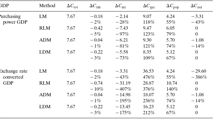
Table 2
Ž .
Decomposition results of the difference in CO emissions BTCO2 2 between world regions in 1993: OECD-FSUrCEE
GDP Method ⌬Ctot ⌬Cfsh ⌬Cint ⌬Cypc ⌬Cpop ⌬Crsd
Purchasing LM 7.67 y0.18 y2.14 9.07 4.24 y3.31
power GDP y2% y28% 118% 55% y43%
Exchange rate LM 7.67 y0.18 y3.31 36.53 4.24 y29.60
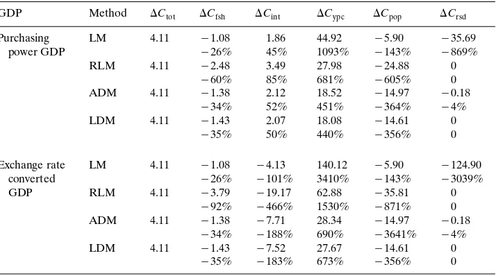
Table 3
Ž .
Decomposition results of the difference in CO emissions BTCO2 2 between world regions in 1993: OECD-ROW
GDP Method ⌬Ctot ⌬Cfsh ⌬Cint ⌬Cypc ⌬Cpop ⌬Crsd
Purchasing LM 4.11 y1.08 1.86 44.92 y5.90 y35.69
power GDP y26% 45% 1093% y143% y869%
RLM 4.11 y2.48 3.49 27.98 y24.88 0
y60% 85% 681% y605% 0
ADM 4.11 y1.38 2.12 18.52 y14.97 y0.18
y34% 52% 451% y364% y4%
LDM 4.11 y1.43 2.07 18.08 y14.61 0
y35% 50% 440% y356% 0
Exchange rate LM 4.11 y1.08 y4.13 140.12 y5.90 y124.90
converted y26% y101% 3410% y143% y3039%
GDP RLM 4.11 y3.79 y19.17 62.88 y35.81 0
y92% y466% 1530% y871% 0
ADM 4.11 y1.38 y7.71 28.34 y14.97 y0.18
y34% y188% 690% y3641% y4%
LDM 4.11 y1.43 y7.52 27.67 y14.61 0
y35% y183% 673% y356% 0
energy intensity of ROW is higher than that of OECD based on exchange-rate-converted GDP but the converse is true when it is based on purchasing power GDP.
The decomposition results given by the four decomposition methods are shown in Tables 2᎐4. The estimated effects are also expressed as percentages of the actual total difference in emissions between regions for ease of comparison. With the same set of emission coefficients used for all regions,⌬Cemc is always zero and is therefore not shown. Residuals for the RLM and LDM are also zero because
Ž
these are perfect decomposition methods. In absolute terms, income effect GDP
.
per capita and population effect are generally the dominant forces leading to different emission levels among the three world regions, while fuel share effect is the smallest.
4. Impacts of variations in explanatory factors
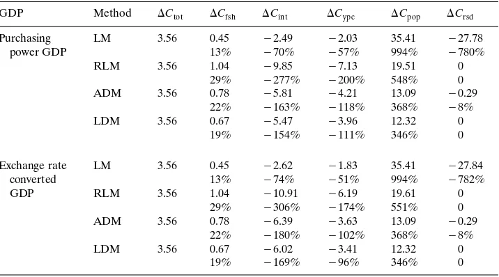
Table 4
Ž .
Decomposition results of the difference in CO emissions BTCO2 2 between world regions in 1993: ROW-FSUrCEE
GDP Method ⌬Ctot ⌬Cfsh ⌬Cint ⌬Cypc ⌬Cpop ⌬Crsd
Purchasing LM 3.56 0.45 y2.49 y2.03 35.41 y27.78
power GDP 13% y70% y57% 994% y780%
Exchange rate LM 3.56 0.45 y2.62 y1.83 35.41 y27.84
converted 13% y74% y51% 994% y782%
As shown in Table 1, the exchange-rate-converted GDP exhibits larger variations as compared to the purchasing power GDP. Residuals given by the LM in the case of exchange-rate-converted GDP are also much larger than those given by purchas-ing power GDP, as shown in Tables 2 and 3. The case of ROW-FSUrCEE decomposition is an exception, as the relative size of their GDP is about the same irrespective of the GDP measure used. Hence for the LM, the magnitude of residual increases with the variations in explanatory factors. Interestingly the residual for the ADM is not affected by how GDP is measured. It can be shown
Ž . Ž .
from Eqs. 5 and 6 that for Divisia-based methods, different GDP measures only
Ž .
affect those effects directly related to GDP, i.e. intensity ⌬Cint and income
Ž⌬Cypc.effects.
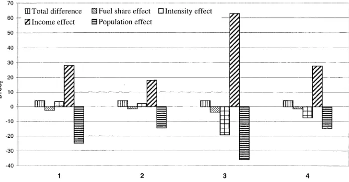
Ž .
Fig. 1. Decomposition results OECD-ROW given by the RLM and the LDM. Plot 1 refers to RLM with purchasing power GDP, plot 2 refers to LDM with purchasing power GDP, plot 3 referes to RLM with exchange-rate-converted GDP, and plot 4 refers to LDM with exchange-rate-converted GDP.
given by the RLM are larger than the corresponding estimates given by the LDM, irrespective of how GDP is measured. It seems that the LDM, which contains logarithmic terms in its formulae, gives more stable decomposition results. In contrast, the RLM tends to introduce greater ‘overlaps’ among effects such that the estimated effects are larger in absolute terms and the degree of cancellation among effects is greater when they are added up to give the actual total change. This is illustrated in a numerical example in the Appendix A, which shows that, when the amplitude of variations in explanatory variables increases, the RLM yields less stable decomposition results as compared to the LDM. It may, therefore, be suggested that the results given by the LDM are more robust than those given by the RDM.
5. Impacts of the choice of GDP measure
Many studies have investigated the problems of using exchange-rate-converted GDP to compare the level of economic activities across countries and in
energy-Ž .
Ž .
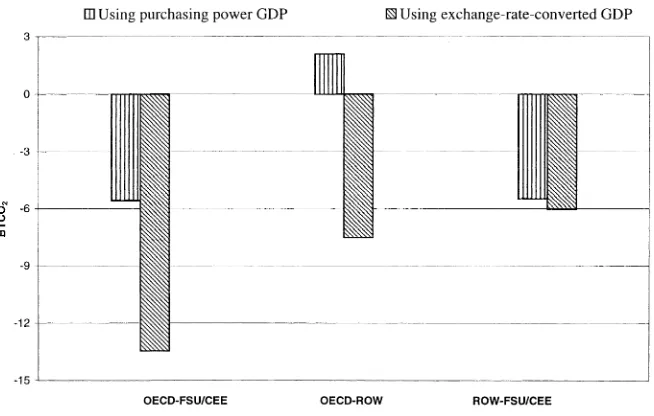
Fig. 2. The estimated intensity effects ⌬Cint given by the LDM using different GDP measures.
switching from exchange-rate-converted GDP to purchasing power GDP in decom-position analysis.
According to the decomposition formulae, the way GDP is measured affects all
Ž
the effects in the RLM but it only affects two GDP-related effects i.e. intensity
.
and income effects in the LDM. Fig. 2 compares the estimates of ⌬Cint given by the LDM using the two different GDP measures. For ROW-FSUrCEE, the estimates are about the same since, as already mentioned, the relative size of their GDP is quite independent of GDP measure. However, in the case of OECD-FSUrCEE, the absolute value of ⌬Cint computed from purchasing power GDP is more than twice that given by exchange-rate-converted GDP. For OECD-ROW, the two measures yield estimates which are opposite in sign. Thus very different conclusions may be reached based on different GDP measures.
6. Structural comparability
cross-country studies as there are often variations among countries in data collec-tion and presentacollec-tion. Hence, adjusting the original data to make them compatible across country is a complication in cross-country decomposition studies. In the
Ž .
study of CO2 emissions by Proops et al. 1993 , the input᎐output tables of Germany and the UK were both aggregated to give consistent production sectors.
Ž .
Similarly, in the study by Chung 1998 , the data for South Korea were modified to make them compatible with those for China and Japan. Generally, as the level of disaggregation increases the need for data adjustments becomes greater. The study by Proops et al. involved 47 economic sectors and that by Chung 45 industrial sectors. In our study, this problem did not arise as structural change involves fuel mix and only six fuel types are studied.
7. Conclusion
Decomposition analysis has been increasingly applied in energy and environmen-tal studies. A recent development has been the application of the technique to cross-countryrregion comparisons. Cross-country decomposition gives rise to sev-eral problems that are often not encountered in chronological decomposition for a specific country. The variations in explanatory factors in the data are very often larger in cross-country decomposition. In such cases, the conventional decomposi-tion methods are no longer effective as they tend to leave a large residual. This not only makes result interpretation difficult but also defeats the purpose of decompo-sition. Due to the superiority of perfect decomposition methods over the conven-tional methods, the former should be adopted in cross-countryrregion decomposi-tion.
We have also shown that the choice of GDP measure can greatly affect decomposition results. For the RLM all effects are affected while for the LDM only those GDP-related effects are affected when a switch is made from one GDP measure to another. Based on this finding and the fact that the LDM gives more stable results as shown in Appendix A, we are inclined to believe that the LDM provides more robust results than those given by the RLM. Nevertheless, this is an issue that deserves further analysis.
Appendix A
We use a simple example to explain why the RLM yields larger values for the quantified effects compared to the LDM. For simplicity consider a two-factor model with only one sector: VsAB. Subscripts 1 and 2 refer to two different
Ž .
countries. Assume A1s␥A2 and B1s 1r␥ B2 where ␥ is a constant. Then
Ž . Ž .
V1sV2sL V1,V2 , where L x,y is the logarithmic mean function. Now we decompose the difference ⌬VsV1yV2 into two components ⌬VAand ⌬VB. For
Ž . Ž . Ž .Ž . Ž .
Ž .
LDM,⌬VAsV2 ln ␥ . The effect ⌬VB is simply the negative value of ⌬VA. Let ␥
vary from 1 and increase multiplicatively in step using a factor of 2. The results
Ž .
obtained are as follows supposeV2s1 :
␥ RLM LMDM
It is clear that as ␥ increases, i.e. the change in the explanatory factor becomes larger, the estimated effect given by the RLM changes at a more rapid rate than that of the LDM. Hence the RLM tends to give greater ‘overlaps’ among the various estimated effects as compared to the LDM. This simple example can partly explain the phenomenon that, for the same effect, the RLM always gives a larger value in absolute terms than that of the LDM, as shown in Tables 2᎐4.
References
Ž .
Ang, B.W., 1987. A cross-sectional analysis of energy-output correlation. Energy Econ. 9 4 , 274᎐286.
Ž .
Ang, B.W., 1995. Decomposition methodology in industrial energy demand analysis. Energy 20 11 , 1081᎐1095.
Ang, B.W., Choi, K.H., 1997. Decomposition of aggregate energy and gas emission intensity for industry:
Ž .
a refined Divisia index method. Energy J. 18 3 , 59᎐73.
Ang, B.W., Zhang, F.Q., 1999. Inter-regional comparisons of energy-related CO emissions using the2
Ž .
decomposition technique. Energy 24 4 , 297᎐305.
Ang, B.W., Zhang, F.Q., Choi, K.H., 1998. Factorising changes in energy and environmental indicators
Ž .
through decomposition. Energy 23 6 , 489᎐495.
Ž .
Birol, F., Okogu, B.E., 1997. Purchasing power parity PPP approach to energy efficiency measurement:
Ž .
implications for energy and environmental policy. Energy 22 1 , 7᎐16.
Boyd, G.A., Hanson, D.A., Sterner, T., 1988. Decomposition of changes in energy intensity-a
compar-Ž .
ison of the Divisia index and other methods. Energy Econ. 10 4 , 309᎐312.
Chung, H.S., 1998. Industrial structural and source of carbon dioxide emissions in east Asia: estimation
Ž .
and comparison. Energy Environ. 9 5 , 509᎐533.
David, P.A., 1972. Just how misleading are official exchange rate conversions. Econ. J. 82, 979᎐990. International Energy Agency, 1997. Energy Environment Update, No. 6, Paris.
OECD, 1997. CO Emissions from Fuel Combustion, 19722 ᎐1995, Paris.
Park, S.H., 1992. Decomposition of industrial energy consumption-an alternative method. Energy Econ.
Ž .
14 4 , 265᎐270.
Proops, J.L.R., Faber, M., Wagenhals, G., 1993. Reducing CO Emissions: A Comparative Input2 ᎐ Out-put Study for Germany and the UK. Springer, Heidelberg.
Raggi, A., Barbiroli, G., 1992. Factors influencing changes in energy consumption: the case of Italy,
Ž .
1975᎐85. Energy Econ. 14 1 , 49᎐56.
Sun, J.W., 1998. Changes in energy consumption and energy intensity: a complete decomposition model.
Ž .