Statistical inference of progressivity dominance: an
application to health care financing distributions
Jan Klavus
∗STAKES, Health and Welfare Economics Group, National Research and Development Centre for Welfare and Health, P.O. Box 220, FIN-00531 Helsinki, Finland
Received 11 November 1999; received in revised form 24 March 2000; accepted 31 July 2000
Abstract
This paper employs a distribution-free statistical test suitable for comparisons based on dependent samples to analyse changes in health care financing distributions on Finnish data. In distinction to the more general summary index approach used in most studies of progressivity measurement, the difference between the Lorenz curve of income inequality and the concentration curves of various taxes and payments is used to evaluate progressivity dominance and changes in progressivity. Sample weights are applied to account for the effect of sampling design and non-response. The analysis demonstrates that the dominance approach can be successfully applied to various types of distributional problems besides comparisons concerning differences in income distributions. As an empirical application the paper presents estimation results for the progressivity of various health care financing sources using data from the 1987 and 1996 Finnish Health Care Surveys. © 2001 Elsevier Science B.V. All rights reserved.
JEL classification:H22; I19
Keywords:Health care finance; Progressivity; Dominance; Statistical tests
1. Introduction
Most of the earlier work on inequality measurement in health care has focused on single valued summary measures of inequality (e.g. Häkkinen, 1992; Wagstaff and van Doorslaer, 1992; Klavus and Häkkinen, 1996; Bishop et al., 1998; Klavus, 1998; Wagstaff et al., 1999). In contrast, the present paper uses the dominance relation between two curves as the criterion for making inequality comparisons.1 The statistical properties of distribution-free Lorenz
∗Tel.:+358-9-3967-2249; fax.:+358-9-3967-2485. E-mail address:[email protected] (J. Klavus).
1If the Lorenz curve of one distribution lies inside that of another the former curve is said to Lorenz dominate
the other.
curve estimates were first documented by Beach and Davidson (1983), who derived a large sample test for Lorenz dominance. Beach and Kaliski (1986) extended the statistical frame-work to weighted samples and recently, Bishop et al. (1994) and Davidson and Duclos (1997) to samples that are not necessarily independently distributed. The two latest contributions have made it possible to test for the relationship between two interdependent curves, with the advantage of being able to analyse the redistributive effect or progressivity of taxes and transfers according to the dominance criterion, in contrast to the more restricted framework provided by single-valued summary measures of progressivity. Besides convenient numeri-cal representation, an obvious advantage of a summary measure is that it allows for cardinal interpretation of the extent of inequality, while the dominance relation enables only inequal-ity rankings of ordinal character. Due to its generalinequal-ity, however, a summary measure can indicate significant progressivity or regressivity in cases, where such outcomes apply only to some part of the income distribution. While the inequality assessment given by the sum-mary measure in such circumstances would not be incorrect, but merely characteristic of its construction, it would certainly yield an imperfect description of the nature of inequality pre-vailing in the distribution. For these reasons, both kinds of analysis are needed for a compre-hensive investigation of income inequality and progressivity at various levels of aggregation. In the context of dominance relations, statistical tests can be constructed to identify pro-gressivity at certain ranges of the income distribution or in the overall distribution. It may also be of interest to consider changes in progressivity over time, to compare different re-gions or demographic groups, or some other independent populations. It should be noted that comparing a Lorenz curve with an associated concentration curve involves a different statistical problem than comparing two independently distributed Lorenz or concentration curves obtained from separate samples. Testing for the former relationship requires in-formation on the asymptotic joint covariance structure of Lorenz and concentration curve ordinates, whereas a test on progressivity changes can be based on the separate sampling distributions of progressivity ordinates estimated from independent samples.
The purpose of the present paper is to apply the above methods to extend the scope of inequality measurement in health care, and to provide support for earlier distributional findings concerning the Finnish health care system (Klavus and Häkkinen, 1998; Klavus, 1998). A methodological extension to earlier work in the tax literature is provided by the use of sample weights in the progressivity analysis. These are specifically estimated quantities indicating the proportion of households or individuals in the population represented by each observation in the sample. Multiplying sample values by sample weights gives an estimate of corresponding quantities at the population level. The weights are constructed to correct for bias arising from non-response or other systematic error sources in the data. The estimation methods presented in this paper can be of particular help for the interested policy analyst being confronted with samples that are available in weighted form only. Moreover, when both unweighted and weighted data are available it is, of course, preferable to use weighted values allowing for the estimation of population averages rather than sample averages. Further, in contrast to previous work, greater effort is placed on consistent treatment of the income unit and the unit of analysis in constructing the size distributions corresponding to relative differences between households, and the income groups.
income inequality and the concentration curve of taxes or other payments. Distribution-free statistical tests are constructed to test for differences in the curves as well as for changes in progressivity over time. Following a description of data and variables in Section 3, a brief overview on the implications of economic changes for the health care system is presented along with the main results concerning progressivity changes and dominance relations. The last section summarises and discusses the findings and the method.
2. Asymptotic inference of progressivity dominance
LetL(p) be the Lorenz curve of income, interpreted as the fraction of total income received by the lowestpth fraction of the population arranged in ascending order of income. The concentration curve of taxes,C(p), is given by the proportion of taxes paid by the lowest
pth fraction of the population. The statistical inference of progressivity involves testing for differences in the ordinates ofL(p) andC(p) at given percentile points,p. In order to conduct the statistical test the joint sampling distribution ofL(p) andC(p) must be known.
Consider a sample of observationsYj for j = 1, . . . , N, ranked in ascending order
of income. Let wj be the weight attached to thejth observation in the sample (j < i
impliesYj < Yi). With sample weights, the proportion of the population represented by
each observation is not necessarily the same and, therefore, weighted ranksRi are defined
as the cumulative sum of weighted observations up to the midpoint of each group interval (cf. Lerman and Yitzhaki, 1989)
Ri = i−1
j=0 wj +
wi
2 (1)
wherewjandwiare the population weights (the aggregate number of people represented by
theith andjth individual in the sample) andw0=0. A relative rank variableri is obtained
by dividing each rank by the sum of the population weights. To construct income groups the ordered sample is partitioned intoKgroups of equal size, so that the sum of relative ranks at the group limits equals or is just less thanpi, wherepi is the abscissaepi =i/K+1
fori=1, . . . , K, corresponding to the income groups. If, for example, deciles are used, K=9 andp1=0.1, . . . , p9=0.9, andriis the closest rank not greater thanpi. Further,
letεyi andεti denote the level of income and tax payments atri.
To establish statistical inference, the first step is to derive the asymptotic distribution of the conditional expectations of income, denoted asγi, and taxes denoted asδi, fori =
1, . . . , K+1. Consider two jointly distributed random variablesYandT. The expectation ofYconditional onribeing less than or equal topi is
γi ≡E[Y|ri ≤pi] (2)
Similarly the conditional expectation ofTatpi is given by
δi ≡E[T|ri ≤pi] (3)
The obvious estimators ofγi andδi in the sample are the weighted cumulative meansγˆi
to the unconditional (weighted) sample meansγˆ andδˆ. From these quantities, the Lorenz curve ordinates can be estimated asΦˆi =pi(γˆi/γ )ˆ , and analogously asΓˆi =pi(δˆi/δ)ˆ for
the concentration curve ordinates.
Let the vector of the conditional means corresponding to the abscissaepi[pi|i=1, . . . , K]
beγγγˆˆˆ ≡(γˆ1, . . . ,γˆK)′andδδδˆˆˆ≡(δˆ1, . . . ,δˆK)′. Progressivity is given by the distance between
each of the ordinate estimates as
ˆ
The asymptotic distribution ofPPPˆˆˆdepends on the joint asymptotic distribution of its terms, represented by a 2(K+1)-vectorθθθˆˆˆ =(p1γˆ1, . . . , pKγˆK,γ , pˆ 1δˆ1, . . . , pKδˆK,δ)ˆ ′. It can
be shown thatθθθˆˆˆis asymptotically normal in that
N (θθθˆˆˆ−θθθ )has a limiting (K+1)-variate normal distribution with mean zero and an asymptotic covariance matrixΩΩΩ(see for example; Beach and Davidson, 1983 and Davidson and Duclos, 1997), where the covariance ofγi
andδj is given by
cov(piγi, pjδj) =pi[E(YiTi)−γiδi+(1−pj)(εyi−γi)(εtj−δj)
+(εyi−γi)(δj−δi)] (5)
The first two terms in brackets denote the covariance ofYandTconditional onri ≤ pi.
The asymptotic covariance ofγiandγj(and forδiandδj by replacingγiwithδi, andεyi
Thus, the matrixΩΩΩ consists of the variance and covariance terms of each ordinate along the curvesL(p) and C(p), and the covariance terms of each ordinate across the curves. Hereafter, shorthands ofγiγjandδiδj are used for the former andγiδjfor the latter terms.
Since the composition of the matrixVVV is rather complex, only the structure of the diagonal terms is presented here. The diagonal terms are
vii =
In order to test for statistical significance of progressivity at an individual ordinatei, the null hypothesisH0:Dˆi =0, whereDˆi = ˆγi/γˆ− ˆδi/δˆ, is tested against the alternative hypothesis
H0:Dˆi =0. Substituting sample estimates for the terms in Eq. (9), the test statistics are
Zi =
ˆ Di
(ˆvii/N )1/2
(10)
which is asymptotically distributed as standard normal. To test for changes in progressivity ordinates estimated from two independent samples, the test statistics is
Zi =
(DˆiA− ˆDBi ) [(ˆvAii/NA)+(vˆB
ii/NB)]1/2
(11)
whereDˆAi andDˆBi refer to two independent progressivity ordinates. For testing the hypoth-esis concerning the dominance relation of entire curves a simultaneous inference approach based on a set of differences at ordinatesi=1, . . . , Kcan be used (see for example; Beach and Richmond, 1985; Bishop et al., 1994). This involves comparing the largest positive and negative values of the individualZ-statistics (Z+,Z−) to the critical value in a studentised
maximum modulus (SMM) table. The test statistics are selected from
Z+=max{0, Zi}; i∈[1, K]; Z−=min{0, Zi}; i∈[1, K] (12)
In the case of two curvesAandB, representing either a Lorenz curve and a concentration curve (i.e. progressivity according to Eq. (10)), or two separate progressivity distributions (i.e. changes in progressivity according to Eq. (11)), the test hypotheses are2
Z+not significant;Z−not significant⇒H0: the two curves are equal Z+significant;Z−not significant⇒H1: A (the reference)dominatesB Z+not significant;Z−significant⇒H2: BdominatesA (the reference) Z+significant;Z−significant⇒H3: the two curves cross
It should be noted that when analysing progressivity or changes in two progressivity distributions the inequality implications of dominance differs from those associated with
2A progressivity distribution is a curve plotting the differences in Lorenz and concentration curve ordinates at
comparisons concerning two Lorenz curves. In the case of Lorenz curves, the dominant (lower) curve always yields less income inequality. In comparisons concerning progressiv-ity, if the Lorenz curve (concentration curve) dominates the concentration curve (Lorenz curve), the tax is progressive (regressive), implying pro-poor (pro-rich) redistribution. When comparing two progressivity distributions referring, for example, to two different time peri-ods the interpretation of dominance is as follows: if the reference distribution is progressive, the dominant curve yields less progressivity (or more regressivity), whereas if the reference distribution is regressive the dominant distribution gives rise to less regressivity (or more progressivity).
3. Data and variables
The estimations were carried out using data from the 1987 and 1996 Finnish Health Care Surveys (FIN-HCS/87 and FIN-HCS/96). These data represent the non-institutionalised population and contain information on the state of health, the use of health services, and households’ medical expenses. In 1987, the sample size was 5858 households giving a total of 16 269 individuals and a response rate of 84.2%. In 1996, the figures were 3614 households, 9037 individuals and an 86.8% response rate. In addition, hospital inpatient data from the Finnish Hospital Discharge Register (FHDR) for 1987 and 1996 were combined with the FIN-HCS data. The FHDR gathers annual data on all public and private hospitals in Finland and it is better suited for examining hospital inpatient utilisation and the distribution of inpatient charges than the survey data which only refers to a 5 months recall period.
In constructing, the weighting variable a post-stratification approach based on age, sex and region was used. Regional age–sex distributions calculated by this method corre-sponded closely to those at the population level. A more detailed description of the followed post-stratification method can be found in Kalimo et al. (1989).
All data on income and taxes were derived from national tax files, except for indirect taxes which were estimated from aggregated household consumption data. The 1985 and 1994–1996 Finnish Household Surveys (FHS) were used for this purpose. The FIN-HCS data were first sorted by income quintile and household type to constitute 5×6 cells, whereafter the incidence of indirect taxes was estimated by weighting consumption in each cell by the value-added and excise tax levies on eight aggregated expenditure groups.3,4 In estimating sickness insurance payments, it was assumed that the employers’ share was borne entirely by employees. Thus, households’ sickness insurance contributions consisted of the payment shares of employers, employees, the state and the municipalities. The contributions of the state and the municipalities were assumed to be borne proportionally to state and municipality taxes.
3The household types were: (1) one-person households; (2) single-parent households; (3) childless couples; (4)
couples with children; (5) elderly households; (6) others.
4Total expenditure consisted of the following items: (1) foodstuffs, beverages and meals; (2) clothing and
Progressivity was analysed with respect to household gross income. All income, taxes and payments were adjusted by an equivalence scale. The OECD-scale was used, in which the first adult receives a weight of 1, every other adult a weight of 0.7, and each child a weight of 0.5. In constituting the income distribution, the individual rather than the household was regarded as the relevant income unit, and correspondingly, individuals were ranked in as-cending order according to their household equivalent gross income. This is analogous to weighting household equivalent income by the number of household members. The weight-ing procedure is in line with individualistic welfare criteria and accounts for differences in the relative size of the household the income units live in (Danziger and Taussig, 1979; Cowell, 1984; Atkinson et al., 1995). When size-deflated household income is weighted by the number of household members income groups should analogously consist of an equal number of persons, not of households, which seems to be the practice followed in most distributional work involving an individualistic approach to inter-household welfare comparisons. In the present study, income deciles were constructed by partitioning the distribution into 10 groups comprising an equal number of persons in each.
Revenues from the following sources were included in the estimation of total health care financing: state income taxes; indirect taxes; local taxes; sickness insurance contributions and households’ out-of-pocket payments. In the absence of earmarked taxes and social in-surance contributions, the proportion of each revenue source used to finance health care is not directly observable. These were estimated by weighting all taxes and sickness insurance contributions by the revenue collecting sector’s share of total health care expenditures. For example, the share of state taxes used to finance health care is equivalent to the state’s share of total health care expenditures. Likewise, the proportions of sickness insurance contri-butions and out-of-pocket payments are equivalent to the expenditure shares of the Social Insurance Institution and direct payments by households, respectively. The tax deduction of medical expenses, which were still permissible in 1987, was considered as an alleviation of households’ actual medical expenses instead of a relief in taxes. This was done in order to maintain uniform basis against which changes in the revenue shares of various financing sectors could be examined despite the abolition of the deduction in 1992. The amount of the benefit depended on the size of the deduction and the marginal tax rate in the recipient households. In order to avoid double-counting the benefit, first in personal income taxation and then in out-of pocket payments, the tax reducing effect of the deduction was estimated and added back to taxable income. This procedure ensured that the distributions of state and local income taxes reflected the tax reducing effect of the deduction, and a corresponding amount could be subtracted from households’ out-of-pocket payments.
4. Results
4.1. Economic trends and structural changes
Fig. 1. Composition of income groups (%) by employment status 1987 and 1996.
private financing, while public expenditure on health care was cut.5 As a consequence of the exceptional economic developments, the demographic composition of income groups changed radically. The percentage of unemployed households rose substantially between 1987 and 1996 (Fig. 1), particularly in the lowest income groups, but also among the better-off households. There was a considerable improvement in the economic situation of the retired population. The proportion of pensioners fell in the three lowest deciles with a corresponding increase in the middle income groups. In addition, the proportion of student households increased in the lowest decile, caused not only by the relative impoverishment of students, but also because in 1996 many unemployed persons registered as students.
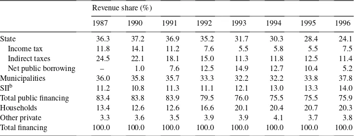
Another structural change with straightforward distributional implications was the shift from public towards private revenue sources in health care financing. As shown in Table 1, the share of households’ out-of-pocket payments increased steadily from 1990 to 1995, while at the same time the share of public financing declined substantially — the development being almost entirely due to a sharp drop in the financing share of the central
5A more detailed description of the changes confronting the health care system is presented in Klavus and
Table 1
Health care financing in Finland 1987 and 1990–1996 (% of total expenditure)a
Revenue share (%)
1987 1990 1991 1992 1993 1994 1995 1996
State 36.3 37.2 36.9 35.2 31.7 30.3 28.4 24.1
Income tax 11.8 14.1 11.2 7.6 5.5 5.8 5.5 7.5
Indirect taxes 24.5 22.1 18.1 15.0 11.3 11.8 12.5 11.4
Net public borrowing – 1.0 7.6 12.5 14.9 12.7 10.4 5.2
Municipalities 36.0 35.8 35.7 33.3 32.2 32.2 33.8 37.8
SIIb 11.2 10.8 11.3 11.1 12.1 13.0 13.3 14.0
Total public financing 83.4 83.8 83.9 79.5 76.0 75.5 75.5 75.9
Households 13.4 12.6 12.6 16.6 20.1 20.4 20.7 20.3
Other private 3.3 3.6 3.5 3.9 3.9 4.1 3.7 3.8
Total financing 100.0 100.0 100.0 100.0 100.0 100.0 100.0 100.0
aSource: health care expenditure and financing in Finland 1960–1996, Social Insurance Institution 1996, and
own calculations.
bSickness Insurance Institution.
government. Private financing peaked in 1995, but an increasing trend towards local revenue sources and the municipalities seems to have prevailed since then.
4.2. Progressivity dominance
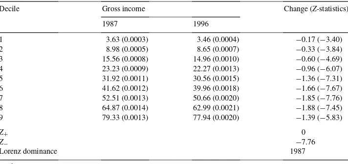
The progressivity of health care financing is not only affected by changes in the financ-ing structure and the incidence of taxes and payments, but also by changes in the income distribution. Comparison of the distribution of gross income across income groups clearly indicated that income inequality increased between 1987 and 1996 (Table 2). The test statistics concerning individual Lorenz ordinates and the entire Lorenz curves showed un-ambiguously that the 1987 curve dominated that of 1996; the individualZ-statistics at each Lorenz ordinate exceeded the critical value at the 95% level, and the largest absolute value corresponding to the simultaneous test statistics,Z+,Z−, exceeded the SMM critical value
atZ∗.
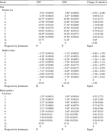
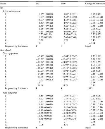
The results concerning progressivity dominance are shown in Table 3. The differences between the Lorenz curve and the concentration curves of various health care financing sources were significant in 1987 and 1996 at all deciles except for the highest deciles for local taxes and sickness insurance payments. Tests on the dominance of entire curves indicated, however, that these financing sources were progressive overall. In addition, the distribution of the income tax emerged progressive, whereas indirect taxes and households’ out-of-pocket payments were clearly regressive.
Table 2
Distribution of gross income at decile ordinates 1987 and 1996a,b
Decile Gross income Change (Z-statistics)
1987 1996
1 3.63 (0.0003) 3.46 (0.0004) −0.17 (−3.40)
2 8.98 (0.0005) 8.65 (0.0007) −0.33 (−3.84)
3 15.56 (0.0008) 14.96 (0.0010) −0.60 (−4.69)
4 23.23 (0.0009) 22.27 (0.0013) −0.96 (−6.07)
5 31.92 (0.0011) 30.56 (0.0015) −1.36 (−7.31)
6 41.62 (0.0012) 39.96 (0.0018) −1.66 (−7.67)
7 52.51 (0.0013) 50.66 (0.0020) −1.85 (−7.76)
8 64.87 (0.0014) 62.99 (0.0021) −1.88 (−7.45)
9 79.33 (0.0013) 77.94 (0.0020) −1.39 (−5.83)
Z+ 0
Z− −7.76
Lorenz dominance 1987
aStandard errors/Z-statistics in parentheses.
bThe SMM critical value ofZ∗(α=0.05,k=9) is 2.77.
progressivity of the income tax and the rather high standard errors for both, the equivalence of the curves in the 2 years could not be rejected in either case. The distribution of local taxes for 1996 lay below that of 1987 at each ordinate, but only at the first decile was the increase in progressivity statistically significant. The distributions of sickness insurance payments were very similar for both years and no changes in progressivity could be observed. Households direct payments, on the other hand, turned out less regressive at lower income levels, but more regressive among the upper deciles. However, the change was significant only at the second decile and the overall statistics concerning the entire curves suggested that the 1996 curve dominated the corresponding curve in 1987 and the apparent crossing of the curves was not supported.
Table 3
Progressivity of health care financing (% difference in the cumulative shares of gross income and health care payments) at decile ordinates 1987 and 1996a,b
Decile 1987 1996 Change (Z-statistics)
State Income tax
1 2.91∗(0.0019) 2.89∗(0.0026) −0.02 (−0.06)
2 6.78∗(0.0043) 6.87∗(0.0060) 0.09 (0.12)
3 10.37∗(0.0073) 10.58∗(0.0103) 0.21 (0.17)
4 13.58∗(0.0106) 14.06∗(0.0146) 0.48 (0.26)
5 15.91∗(0.0141) 17.10∗(0.0200) 1.19 (0.49)
6 17.89∗(0.0175) 19.34∗(0.0254) 1.45 (0.47)
7 19.03∗(0.0211) 19.82∗(0.0313) 0.79 (0.21)
8 18.05∗(0.0245) 19.29∗(0.0377) 1.24 (0.28)
9 14.88∗(0.0269) 15.50∗(0.0424) 0.62 (0.12)
Z+ 15.77 11.45 0.49
Z− 0 0 −0.06
Progressivity dominance P P Equal
Indirect taxes
1 −2.72∗(0.0014) −3.12∗(0.0022) −0.40 (−1.55) 2 −4.24∗(0.0030) −5.23∗(0.0051) −0.99 (−1.69) 3 −5.40∗(0.0052) −6.76∗(0.0087) −1.36 (−1.34) 4 −6.23∗(0.0074) −7.83∗(0.0124) −1.60 (−1.11) 5 −6.82∗(0.0106) −8.83∗(0.0177) −2.01 (−0.97) 6 −7.15∗(0.0122) −9.47∗(0.0217) −2.32 (−0.93) 7 −7.21∗(0.0146) −9.65∗(0.0265) −2.44 (−0.81) 8 −6.90∗(0.0170) −9.28∗(0.0321) −2.38 (−0.66) 9 −5.66∗(0.0188) −7.33∗(0.0363) −1.67 (−0.41)
Z+ 0 0 0
Z− −19.43 −14.18 −1.69
Progressivity dominance R R Equal
Municipalities Local tax
1 1.33∗(0.0013) 1.85∗(0.0014) 0.52 (2.72)
2 2.74∗(0.0027) 3.19∗(0.0031) 0.45 (1.09)
3 3.27∗(0.0044) 3.85∗(0.0051) 0.58 (0.86)
4 3.27∗(0.0062) 4.00∗(0.0075) 0.73 (0.75)
5 3.11∗(0.0090) 3.95∗(0.0114) 0.84 (0.58)
6 2.78∗(0.0101) 3.65∗(0.0129) 0.87 (0.53)
7 2.30 (0.0121) 2.91 (0.0158) 0.61 (0.31)
8 1.43 (0.0140) 2.03 (0.0191) 0.60 (0.25)
9 0.60 (0.0154) 0.96 (0.0214) 0.36 (0.14)
Z+ 10.23 13.21 2.72
Z− 0 0 0
Table 3 (Continued)
Decile 1987 1996 Change (Z-statistics)
SII
Sickness insurance
1 1.75∗(0.0019) 1.88∗(0.0021) 0.13 (0.46)
2 3.79∗(0.0045) 3.43∗(0.0050) −0.36 (−0.54)
3 5.03∗(0.0077) 4.43∗(0.0085) −0.60 (−0.52)
4 5.53∗(0.0111) 4.90∗(0.0123) −0.63 (−0.38)
5 5.55∗(0.0149) 5.21∗(0.0173) −0.34 (−0.15)
6 5.18∗(0.0183) 5.24∗(0.0214) 0.06 (0.02)
7 4.39∗(0.0221) 4.68 (0.0264) 0.29 (0.08)
8 3.25 (0.0256) 3.95 (0.0319) 0.70 (0.17)
9 1.87 (0.0285) 2.65 (0.0360) 0.78 (0.17)
Z+ 9.21 8.95 0.46
Z− 0 0 −0.54
Progressivity dominance P P Equal
Households Direct payments
1 −7.40∗(0.0054) −6.04∗(0.0047) 1.36 (1.90)
2 −13.27∗(0.0071) −10.48∗(0.0071) 2.79 (2.78)
3 −17.22∗(0.0161) −14.02∗(0.0129) 3.20 (1.55)
4 −17.61∗(0.0121) −15.93∗(0.0116) 1.68 (1.00)
5 −18.29∗(0.0142) −17.11∗(0.0156) 1.18 (0.56)
6 −17.09∗(0.0167) −16.94∗(0.0193) 0.15 (0.06)
7 −14.68∗(0.0194) −15.14∗(0.0224) −0.46 (−0.16) 8 −11.76∗(0.0220) −12.95∗(0.0251) −1.19 (−0.36) 9 −7.77∗(0.0240) −8.06∗(0.0285) −0.29 (−0.08)
Z+ 0 0 2.78
Z− −18.69 −14.76 −0.36
Progressivity dominance R R 1996
Total payments
1 −0.85∗(0.0012) −0.63∗(0.0014) 0.18 (0.98)
2 −0.97∗(0.0019) −0.87∗(0.0024) 0.10 (0.33)
3 −1.13∗(0.0034) −1.17∗(0.0037) −0.04 (−0.08) 4 −0.96∗(0.0039) −1.30∗(0.0047) −0.34 (−0.56)
5 −0.99 (0.0066) −1.40 (0.0086) −0.41 (−0.38)
6 −0.81 (0.0061) −1.34 (0.0078) −0.53 (−0.54)
7 −0.56 (0.0072) −1.24 (0.0094) −0.68 (−0.57)
8 −0.57 (0.0083) −1.15 (0.0115) −0.58 (−0.41)
9 −0.45 (0.0088) −0.67 (0.0130) −0.22 (−0.14)
Z+ 0 0 0.98
Z− −7.08 −4.50 −0.57
Progressivity dominance R R Equal
aStandard errors/Z-statistics in parentheses.
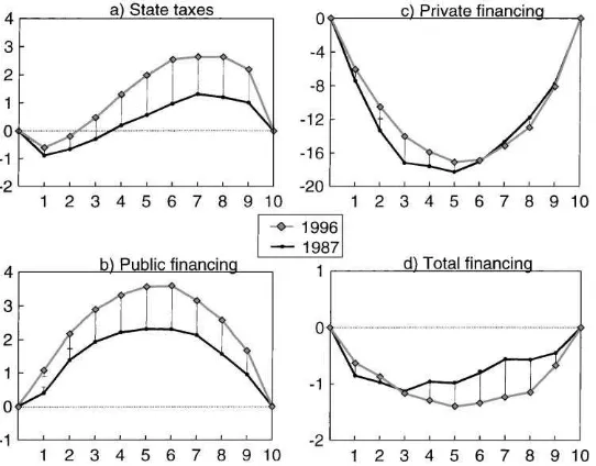
Fig. 2. Progressivity of health care financing (% difference in the cumulative shares of gross income and health care payments) by income deciles, 1987 and 1996 with 95% upper/lower confidence intervals (solid line: crossing error bars).
5. Findings and conclusions
The main contribution of the paper was to establish statistical inference of progressivity dominance involving samples that are not necessarily independently distributed, and to show how the approach can be applied to distributional issues concerning the health care system. The paper also emphasised the use of sample weights and an appropriate choice of the unit of analysis in the construction of income groups. It was shown that assessment of the dominance relation between the Lorenz curve of income inequality and the concentration curve of tax payments reveals certain features of inequality that cannot be observed in an analysis based solely on summary measures, such as the progressivity index. As suggested by the results concerning the distribution of various health care financing sources, the distributional outcome associated with the entire curve does not necessarily conform to individual parts of it, and consequently, the distribution of taxes and payments may at certain income levels be exactly opposite to that indicated by a summary measure of progressivity. The analysis also indicated that taking into account the dependent structure of the income and payment variables and with the rather small sample size used in the analysis, changes in progressivity were often too small to account for any significant differences in the curves.
State taxes emerged progressive except at the lowest income levels, which must be due to the poor earnings of the lowest income decile and the fact that the composition of the income groups changed during the recession — working aged people suffered from unemployment and lower real income levels, whereas pensioners improved their relative position through better pension yields and by not experiencing unemployment. As the proportion of retired and elderly households in the middle income groups grew and the lower income groups consisted increasingly of younger and healthier households, the pattern of health care utilisation and the distribution of out-of-pocket payments shifted towards the middle income groups. This development contributed to emergence of out-of-pocket payments as less regressive in 1996 in spite of the substantial increases in cost-sharing that took place between 1987 and 1996.
While computationally more involved, statistical inference applied to dominance relations provides a useful extension to summary indices in inequality measurement, and allows for a more disaggregated examination of the structure of inequality. Progressivity dominance, derived in the present study, also serves as a generalisation for most previous statistical inference findings concerning quantile-based estimators of inequality. Moreover, it provides the statistical basis for assessing horizontal inequity and redistribution within the dominance framework.
Despite the normative content attached to dominance relations in welfare economics, the approach adopted in this study was mainly descriptive. It can be shown that under rather general conditions of the form of the social welfare function, a progressive tax yields higher social welfare than a proportional tax applied to the same pre-tax income distribution. The same applies to inequality reducing changes in the pre-tax income distribution if progressiv-ity remains fixed. However, these properties translate to comparisons concerning changes in the degree of progressivity only under very special conditions, requiring a certain form of the social welfare function and a progressivity index to be specified. In the sense of utilising the above properties, the assessment of the dominance relation between two mean adjusted pre-tax and after-tax distributions could provide a useful generalisation, allowing the iden-tification of welfare implications and inequality orderings similar to those associated with Lorenz dominance.
References
Atkinson, A., Rainwater, L., Smeeding, T., 1995. Income Distribution in OECD Countries: Evidence from the Luxembourg Income Study. OECD Social Policy Studies #18.
Beach, C.M., Davidson, R., 1983. Distribution-free statistical inference with Lorenz curves and income shares. Review of Economic Studies 50, 723–735.
Beach, C.M., Kaliski, S.F., 1986. Lorenz curve inference with sample weights: an application to the distribution of unemployment experience. Applied Statistics 35, 38–45.
Beach, C., Richmond, J., 1985. Joint confidence intervals for income shares and Lorenz curves. International Economic Review 26, 439–450.
Bishop, J.A., Chow, K.V., Formby, J.P., 1994. Testing for marginal changes in income distributions with Lorenz and concentration curves. International Economic Review 35, 479–488.
Bishop, J.A., Formby, J.P., Zheng, B., 1998. Inference tests for Gini-based tax progressivity indexes. Journal of Business and Economic Statistics 16, 322–330.
Danziger, S., Taussig, M., 1979. The income unit and the anatomy of income distribution. Review of Income and Wealth 25, 365–375.
Davidson, R., Duclos, J.-Y., 1997. Statistical inference for the measurement of the incidence of taxes and transfers. Econometrica 65, 1453–1465.
Häkkinen, U., 1992. Health care utilisation, health and socioeconomic equality in Finland. Sosiaali ja terveyshallitus, Tutkimuksia 20, Valtion painatuskeskus (in Finnish).
Kalimo, E., Klaukka, T., Lehtonen, R., Nyman, K., 1989. Health security in Finland and needs for development. Main results of a nationwide health security survey conducted in 1987. Publications of the Social Insurance Institution, Finland, M:81, Helsinki.
Klavus, J., 1998. Progressivity of health care financing: estimation and statistical inference. Finnish Economic Papers 11, 86–95.
Klavus, J., Häkkinen, U., 1996. Health care and income distribution in Finland. Health Policy 38, 31–43. Klavus, J., Häkkinen, U., 1998. Micro-level analysis of distributional changes in health care financing in Finland.
Journal of Health Services Research and Policy 3, 23–30.
Lerman, R.I., Yitzhaki, S., 1989. Improving the accuracy of estimates of Gini coefficients. Journal of Econometrics 42, 43–47.
Rao, R.C., 1973. Linear Statistical Inference and Its Applications. Wiley, New York.
Wagstaff, A., van Doorslaer, E., 1992. Equity in the finance of health care: some international comparisons. Journal of Health Economics 11, 361–387.