Size economies and optimal scheduling in
shrimp production: results from a computer
simulation model
X. Tian
a, P.S. Leung
b,*, D.J. Lee
c aDepartment of Business,Economic De6elopment and Tourism,HI,USA
bDepartment of Molecular Biosciences and Biosystems Engineering,Uni
6ersity of Hawaii at Manoa,
3050Maile Way,Gilmore Hall111,Honolulu,HI96822,USA
cDepartment of Food and Resource Economics,Institute of Food and Agricultural Sciences, Uni6ersity of Florida,FL,USA
Received 10 October 1999; accepted 14 March 2000
Abstract
This paper describes a computer simulation model developed to analyze the economics of shrimp production under different stocking regimes, harvesting schedules, and farm sizes. The operation examined is ‘closed-market’ where all stages of production occur on-site, and the final product, adult shrimp, are sold in the market. The model was parameterized using existing market data and secondary production data collected from experimental units at the Oceanic Institute in Hawaii. Results indicated that a weekly stocking and harvesting regime is more profitable than either a biweekly or 8-week stocking and harvesting regime. Scale economies indicated that the minimum farm size is twenty-six growout ponds and the optimal farm size is 64 growout ponds. © 2000 Elsevier Science B.V. All rights reserved.
Keywords:Shrimp production; Size economies; Optimal scheduling; Simulation model
www.elsevier.nl/locate/aqua-online
1. Introduction
In intensive shrimp production, shrimp (L.6annamei) are reared in four distinct
stages (maturation, hatchery, nursery, and growout) corresponding to the four life
Senior authorship is not assigned.
* Corresponding author. Tel.: +1-808-9568562; fax:+1-808-9569269. E-mail address:[email protected] (P.S. Leung)
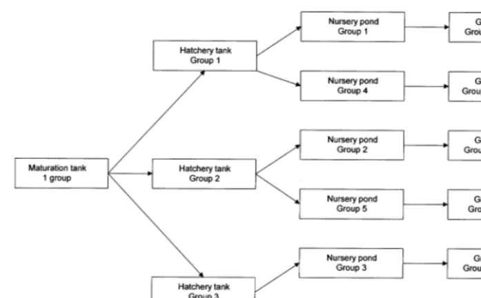
phases of the animal (nauplii, post-larvae, juvenile, and adult). In a closed-market system, all rearing from nauplii production to adult occurs at the same facility. Thus, production of the final marketable output, adult animals, is completely dependent on the rearing of all three precursor stages of production. To assure sufficient input into subsequent stages of production, it may make economic sense to produce an abundance of nauplii, for example, and dispose of the excess. An illustration of a general, closed-market operation withn-stages and free disposal is shown in Fig. 1.
In producing a desired level of final output, a farmer may wish to determine the amount of intermediate product needed at each stage to generate the least amount of waste, i.e. the least cost method of production. To find the least cost method, the economic approach specifies a series of production cost functions needed to capture the scope economies and size economies of the operation. The scope economies are the cost savings derived from producing several products simultaneously from sharing fixed inputs (such as vehicles, buildings, and employees) which are used interchangeably in more than one stage of production (Baumol et al., 1988). Size economies occur when average cost (total cost per unit of shrimp) changes with output level. If shrimp price is constant in output level, then ideally, a farmer may choose to increase (or decrease) the size of the operation to minimize average cost. This paper examines operation size and scheduling decisions in shrimp production using an economic computer simulation model. The remainder of the paper is organized as follows. Section 2 describes the components of the shrimp farm model and the data used to parameterize the model. Section 3 lays out the scenarios analyzed. Section 4 presents the model results and concludes the paper.
Fig. 2. Relationship between groups of production phases.
2. Shrimp farm model
In practice, the primary objective of a shrimp farming operation can vary from maximizing total production, to minimizing downside risk, to meeting delivery agreements, to maximize farm profits, or a combination of these objectives. For simplicity, we assume that the shrimp farmer operates to maximize long-run farm profits subject to input constraints. Our shrimp farmer receives a fixed unit price for any amount of shrimp produced and can access all the resource inputs necessary to expand farm size without limit. Shrimp reproduction and growth rates are assumed known and fixed. A single production technology is available to the farmer. The cost of this technology is known and fixed. The farmer thus is left to make the following joint production decision. How large (number of ponds) should the farm be? And with what frequency should the ponds be restocked each year?
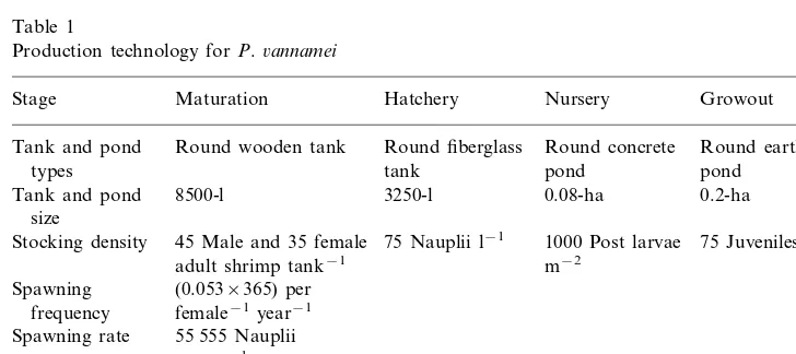
2.1.Production technology
nursery ponds until they form a carapace, then moved to growout ponds where they are reared to a marketable weight. The production technology and stocking densities of the intensive shrimp operation described here are displayed in Table 1 and are largely based on the protocol developed at the Oceanic Institute in Hawaii (Wyban and Sweeney, 1991).
2.2.Model equations
Annual farm profit p is defined to be total revenue (TR) less total cost (TC):
p=TR−TC (1)
Total revenue is price per unit output multiplied by the quantity of shrimp produced:
TR=P×Q (2)
Annual shrimp productionQis a function of number of growout ponds (G), size of the pond (S), stocking density of the pond (D), survival rate (R), and number of cycles per year (t).
Q=f(G, S, D, R,t) (3)
Total annual cost of production (TC) include both fixed (FC) and variable costs (VC):
TC=FC+VC (4)
Costs include resource inputs, labor, and depreciated capital. Fixed and variable cost functions for an intensive shrimp farm operation were estimated by Tian
Table 1
Production technology forP.6annamei
Growout Hatchery Nursery
Stage Maturation
Round concrete
Tank and pond Round wooden tank Round fiberglass Round earth
pond pond
types tank
3250-l
Tank and pond 8500-l 0.08-ha 0.2-ha
size
75 Juveniles m−2 75 Nauplii l−1
Stocking density 45 Male and 35 female 1000 Post larvae m−2
adult shrimp tank−1 Spawning (0.053×365) per
female−1year−1 frequency
Spawning rate 55 555 Nauplii spawn−1
85%
Survival rate 56% 90%
15 weeks Cycle duration 1 day 16 days 5 weeks
Outdoor
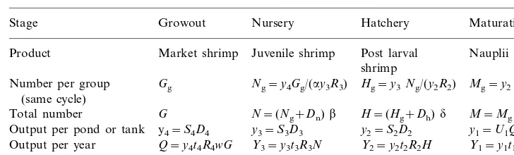
Table 2
Identity equations and constraints
Hatchery Maturation Nursery
Stage Growout
Juvenile shrimp
Market shrimp Post larval
Product Nauplii
(1993) and are as follows. Fixed cost (FC) as a function of the number of maturation tanks (M), hatchery tanks (H), nursery ponds (N) and growout ponds (G) is:
FCc=35.8140+5.9768M+3.0964H+6.0632N+6.9669G−0.0014M 2
−0.0023H2−0.0130N2−0.0097G2 (5)
Variable cost (VC) as a function of the number of maturation tanks (M), hatchery tanks (H), nursery ponds (N) and growout ponds (G), and their respec-tive number of cycles per year (t1, t2, t3, and t4) is:
VC=((0.3653+0.0494M)t1+(6.3216+0.4534H)t2+(22.6640+2.0046N)t3
+(61.1774+19.8060G)t4)103
(6)
The identity equations (Table 2) provide the linking relationships between the four stages of production. Definitions of the model variables can be found in Appendix A.
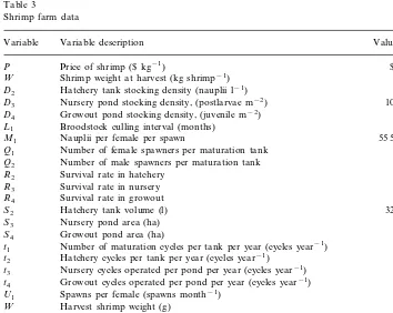
2.3.Data 6alues
The model was parameterized using the data displayed in Table 3.
3. Model scenarios
Three model scenarios were developed to capture a plausible range of farm sizes for evaluating scale economies in shrimp production and are described in Section 3.1 – Section 3.3.
3.1.Growout ponds are stocked and har6ested weekly
A shrimp farm with as few as 16 growout ponds can harvest marketable shrimp weekly. Each pond will be restocked and harvested three times per year for a total of 48 harvests, about one per week. A production schedule is displayed in Fig. 3.
3.2.Growout ponds are stocked and har6ested biweekly
A shrimp farm with as few as eight growout ponds can harvest marketable shrimp every other week. Each pond will be restocked and harvested three times per year for a total of 24 harvests, twice per month. A production schedule is displayed in Fig. 4.
Shrimp weight at harvest (kg shrimp−1)
W 0.023
75 Hatchery tank stocking density (nauplii l−1)
D2
1000 D3 Nursery pond stocking density, (postlarvae m−2)
D4 Growout pond stocking density, (juvenile m−2) 75
Broodstock culling interval (months) 3
L1
Nauplii per female per spawn
M1 55 555
Number of female spawners per maturation tank
Q1 35
Q2 Number of male spawners per maturation tank 45
R2 Survival rate in hatchery 0.56
Survival rate in nursery 0.85
R3
R4 Survival rate in growout 0.9
Hatchery tank volume (l)
S2 3250
0.08 S3 Nursery pond area (ha)
Growout pond area (ha)
S4 0.2
t1 Number of maturation cycles per tank per year (cycles year−1) 48 Hatchery cycles per tank per year (cycles year−1)
t2 18
t3 Nursery cycles operated per pond per year (cycles year−1) 9 3 Growout cycles operated per pond per year (cycles year−1)
t4
U1 Spawns per female (spawns month−1) 1.59
Harvest shrimp weight (g) 23
W
Nauplii per tank (nauplii cycle−1) 103 055 y1
243 750 Postlarvae per tank (postlarvae cycle1)
y2
Juvenile per pond (juvenile cycle1) 800 000 y3
150 000 Shrimp per pond (adult shrimp cycle1)
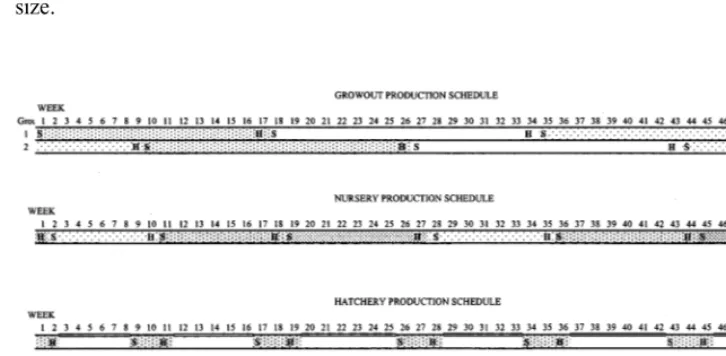
Fig. 3. Closed-market operational system production schedule — growout ponds are stocked weekly.
3.3.Growout ponds are stocked and har6ested e6ery 8 weeks
A shrimp farm with as few as two growout ponds will allow for a harvest of 23 g shrimp every 8 weeks. At this rate, the ponds must be restocked and harvested three times per year for a total of six harvests, or one every 2 months. A production schedule is displayed in Fig. 5.
3.4.Parameter 6alues for the model scenarios
The parameter values for the three stocking and harvesting scenarios, once per week, biweekly, and every 8 weeks, are shown in Table 4.
4. Results and discussions
4.1.Growout ponds are stocked and har6ested weekly
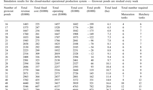
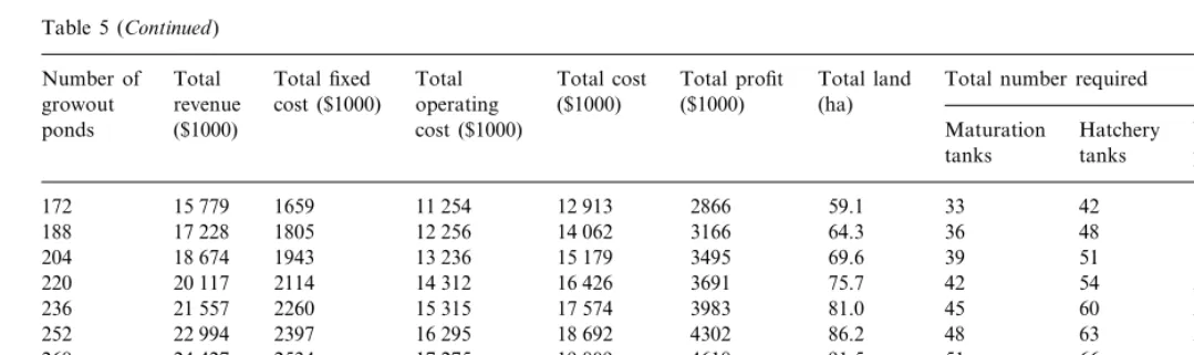
The simulation results under weekly growout schedule are presented in Table 5, and the size economy is depicted in Fig. 6. Table 5 shows that farms with 25 growout ponds or less under this production schedule are not profitable. Fig. 6 provides a graphical representation of size economy showing the ratio of cost over revenue versus farm size. It indicates that farms with 140 ponds would capture most of the size economy meaning that there will not be much cost savings when increasing farm size beyond 140 growout ponds. The L-shaped size economy curve indicates that average cost is constant for a wide range of farm size.
Table 4
Parameter values for the three stocking and harvesting scenarios
Parameter Stocking and harvesting schedule scenarios 3.3 (8 week) 3.2 (bi-weekly)
3.1 (weekly)
1 16
a(minimum number of growout ponds) 8 3
b(minimum number of nursery ponds) 6 1
3 2 1
d(minimum number of hatchery tanks)
3 3
3 t1(number of maturation cycles per tank
per year)
9 9
t2(hatchery cycles per tank per year) 6
6 t3(nursery cycles operated per pond per 18 12
year
6
48 25
t4(growout cycles operated per pond per year)
]16 ]8
G(total number of growout ponds) ]2
]1
]3 N(total number of nursery ponds) ]6
]1 H(total number of hatchery tanks) ]3 ]2
]1 ]1
M(total number of maturation tanks) ]1
X
Simulation results for the closed-market operational production system — Growout ponds are stocked every week Total fixed Total Total land Total number required Total
Number of Total cost Total profit C/R ratio
(ha)
1483 225 1457 6 1.13
16 1682 −199
19 1760 261 1647 1908
7.5 6 7 6 1.07
20 1853 268 1707 1975 −122
7.8 6 7 6 1.05
−96
21 1945 275 1766 2041
8.1 6 7 6 1.03
22 2038 282 1825 2108 −70
8.4 6 8 6 1.03
−54
2185
23 2130 292 1892
8.8 6 8 6 1.01
24 2223 299 1952 2251 −28
9.1 6 9 6 1.01
−12
25 2316 309 2019 2328
9.4 6 9 6
26 2408 316 2078 2394 14 0.99
9.7 6 9 6 0.98
40 2461
27 2501 323 2138
10.1 6 9 6 0.97
28 2594 330 2197 2527 66
10.4 6 9 6 0.97
93
29 2686 337 2257 2593
10.7 6 9 6 0.96
30 2779 344 2316 2660 119
11.0 6 9 6 0.95
145 2726
31 2871 351 2375
11.4 7 9 6 0.95
32 2963 364 2437 2801 162
14.0 8 12 6 0.91
331
40 3702 435 2937 3372
16.6 10 12 6 0.88
48 4440 502 3417 3919 521
20.6 12 15 6 0.86
782
60 5546 607 4157 4763
26.7 15 21 12 0.86
76 7017 789 5256 6044 973
31.9 18 24 12 0.84
1323
92 8485 927 6236 7162
37.2 21 27 12 0.83
108 9950 1065 7215 8280 1670
42.5 24 33 12 0.83
1983 9430
124 1412 1212 8218
47.7 27 36 12 0.82
140 12 871 1350 9198 10 547 2324
53.8 30 39 18 0.82
2531
299
Table 5 (Continued)
Total fixed Total Total land Total number required Total
Number of Total cost Total profit C/R ratio
(ha)
172 12 913 2866
4.2.Growout ponds are stocked and har6ested biweekly
The simulation results under the bi-weekly schedule are presented in Table 6 and Fig. 7. Similar to the weekly schedule, farms are profitable if farm size reaches 26 ponds. Farms with 100 growout ponds would capture most of the economies of size.
4.3.Growout ponds are stocked and har6ested e6ery 8 weeks
The simulation results under the 8 weeks growout stocking and harvesting strategy are presented in Table 7 and Fig. 8. The results indicate that it is generally not profitable under this production strategy. Size economy can be captured around 30 ponds but the profits are negative even up to 40 ponds.
4.4.Discussion
In comparing the profitability of the production schedules, it can be seen that the weekly schedule would generate more profit than the biweekly schedule for farms with the same number of growout ponds. For example, a farm with 48 ponds can generate an estimated net profit of $520 800 with a weekly schedule and $394 000 with the biweekly schedule.
301
Simulation results for the closed-market operational production system — Growout ponds are stocked every 2 weeks Total fixed Total Total land Total number required Total
Number of Total cost Total profit C/R ratio
(ha)
18 1667 239 1563 1803
6.8 8 8 3 1.08
19 1759 258 1635 1893 −135
7.1 8 8 3 1.06
−109
20 1851 265 1694 1960
7.5 8 8 3 1.04
21 1944 272 1754 2026 −82
7.8 9 8 3 1.03
−64
2100
22 2036 285 1814
8.1 9 8 3 1.02
23 2128 292 1874 2166 −38
8.5 10 8 3 1.01
−20
24 2220 305 1935 2240
8.8 10 10
25 2312 318 2005 2323 −11 3 1.00
9.1 10 10 3 0.99
15 2389
26 2405 325 2064
9.5 11 10 3 0.99
27 2496 338 2125 2463 34
9.8 11 10 3 0.98
60
28 2589 345 2184 2529
10.1 11 10 3 0.97
29 2681 352 2244 2596 86
10.5 12 10 3 0.96
104 2669
30 2773 365 2304
10.8 12 12 3 0.96
31 2865 378 2375 2753 113
11.2 13 12 3 0.96
131
32 2957 391 2435 2826
14.3 16 14 6 0.94
40 3692 488 2973 3462 230
16.9 19 16 6 0.91
395
48 4426 568 3463 4031
19.6 22 20 6 0.90
56 5158 653 3964 4617 540
22.3 25 22 6 0.88
701
64 5888 733 4454 5187
25.0 28 24 6 0.87
72 6617 812 4944 5756 861
28.1 31 26 9 0.87
953 6391
80 7344 909 5482
30.7 34 30 9 0.86
88 8070 994 5983 6977 1093
33.4 37 32 9 0.86
1248
X
Table 6 (Continued)
Number of Total Total fixed Total Total cost Total profit Total land Total number required C/R ratio ($1000)
ponds ($1000) cost ($1000) Hatchery Nursery
tanks tanks ponds
8115 1402 36.1 40 34 9 0.85
9517
104 1152 6963
39.2 43 38 12 0.86
112 1238 1255 7512 8766 1471
41.9 46 40 12 0.85
1622
120 10 957 1334 8002 9335
44.6 49 42 12 0.85
128 11 675 1413 8492 9904 1771
47.2 52 44 12 0.85
1918
136 12 391 1492 8981 10 473
303
Simulation results for the closed-market operational production system — Growout ponds are stocked every 8 weeks
Total fixed Total C/R ratio
Total Total cost Total profit Total land Total number required Number of
ponds ($1000) cost ($1000) Hatchery Nursery
tanks tanks ponds
12 406 1163 1569
−494
18 1638 583 1559
9.1 61 26 5 1.29
20 1816 643 1697 2340 −524
9.9 67 29 5 1.27
−533
22 1994 701 1826 2527
−561
26 819 2093 2912
−595
32 2868 999 2500 3499
15.3 03 44 8 1.21
34 3041 1053 2626 3679 −639
16.2 109 47 8 1.20
−652
36 3213 1110 2755 3865
4068 −685 17.2 115 50 9 1.20
38 3384 1172 2896
18.0 121 52 9 1.20
−694
1226
Fig. 8. Economies of size for shrimp farming under the closed-market operational production system — Growout ponds are stocked every 8 weeks.
Weekly stocking and harvesting of growout ponds is a more efficient operation, in terms of production unit (tanks and ponds) utilization, than the biweekly schedule. Weekly schedule would use all the maturation tanks, hatchery tanks, and nursery ponds almost every week. Biweekly stocking would use all the nursery ponds almost every week, but the maturation and hatchery tanks are not fully used. The hatchery tanks stay idle for one third of the time in a year and the maturation tanks are not in use for more than half of the time in a year.
For growout ponds of 0.2 ha in size with a stocking density of 75 juveniles/m2,
For the purpose of comparison, profitability of each phase of the shrimp operation was analyzed as if they were independently operated, i.e. markets exist for nauplii, postlarvae and juveniles. The following market prices were assumed: nauplii at $1 per 1000, postlarvae at $9 per 1000, juveniles at $20 per 1000, and market-size shrimps at $10 per kg. Under such conditions, an independent matu-ration facility would need to have 52 tanks in order to be profitable. On the other hand, it would only take 21 hatchery tanks, five nursery ponds, and nine growout ponds to be profitable if they were operated independently. In other words, while it would require a fairly large size of operation for a profitable maturation facility, relatively small profitable independent operations can be achieved for hatchery, nursery, and growout. While it would require at least 26 growout ponds to achieve positive profits for a closed system, only nine growout ponds would be necessary if juveniles were available at the assumed prices. The analysis seems to indicate that it would be more profitable for shrimp farms to purchase juveniles and postlarvae than to produce their own under current mar-ket conditions. Of course, vertically integrated farms would be preferable if supply of juveniles and postlarvae were inconsistent both in terms of availability and quality. However, as demonstrated in the above analysis, such farms would generally have to be larger.
It should be noted that the assumed growout production protocols as prac-ticed at the Oceanic Institute are rather intensive and they are not commonly practiced in the shrimp industry. Thus, the results with respect to the minimal and optimal farm sizes are only applicable to such intensive systems. While the results presented are specific for the intensive growout system, the methodology developed can be used to evaluate a wide-range of commercial facilities; to determine optimal farm size and to reveal gains from integrating production phases. Nevertheless, the results presented do support the observed small and fragmented rather than vertically integrated shrimp industry particularly in Asia.
Acknowledgements
The authors are indebted to Dr James A. Wyban for providing the necessary bio-technical details of the various phases of shrimp mariculture; and the three anonymous journal reviewers for their constructive comments. This research was supported by the US Department of Agriculture under CSRS Special Grant managed by the Pacific Basin Advising Group.
Appendix A. Nomenclature
annual profit ($) p
total revenue ($) TR
annual shrimp production (kg)
Q
shrimp weight at harvest (kg shrimp−1)
D2 hatchery tank stocking density (nauplii l−1)
nursery pond stocking density, (postlarvae m−2) D3
growout pond stocking density, (juvenile m−2) D4
number of growout ponds per group
Gg
total number of growout ponds
G
number of hatchery tanks per group
Hg
number of hatchery tanks in all the groups
H
L1 broodstock culling interval (months) nauplii per female per spawn
M1
number of maturation tanks per group
Mg
number of maturation tanks in total
M
number of nursery ponds per group
Ng
number of nursery pond in total
N
number of female spawners per maturation tank
Q1
number of male spawners per maturation tank
Q2
R2 survival rate in hatchery survival rate in nursery
R3
survival rate in growout
R4
hatchery tank volume (l)
S2
S3 nursery pond area (ha) growout pond area (ha)
S4
number of maturation cycles per tank per year (cycles year−1) t1
t2 hatchery cycles per tank per year (cycles year−1)
nursery cycles operated per pond per year (cycles year−1) t3
growout cycles operated per pond per year (cycles year−1) t4
spawns per female (spawns month−1) U1
harvest shrimp weight (g)
W
minimum number of growout ponds a
minimum number of nursery ponds b
minimum number of hatchery tanks d
nauplii per tank (nauplii cycle−1) y1
postlarvae per tank (postlarvae cycle−1
)
y2
juvenile per pond (juvenile cycle−1
)
y3
shrimp per pond (adult shrimp cycle−1
)
y4
annual maturation production (nauplii)
Y1
annual hatchery production (post larvae)
Y2
annual nursery production (juveniles)
References
Baumol, W.J., Panzar, J.C., Willig, R.D., 1988. Contestable Markets and the Theory of Industry Structure. Harcourt Brace Jovanovich, Florida, 538pp.
Tian, Xijun, 1993. Optimal Aquafarm Structure and Size: A Case Study of Shrimp Mariculture. Unpublished Ph.D. Dissertation. University of Hawaii at Manoa, Monoa, Hawaii, 179pp. Wyban, J.A., Sweeney, J.N., 1991. Intensive Shrimp production Technology: The Oceanic Institute
Shrimp Manual. The Oceanic Institute, Hawaii, 158pp.