Aquacultural Engineering 22 (2000) 243 – 254
Optimizing multi-stage shrimp production
systems
Jaw-Kai Wang
a,* , Junghans Leiman
baDepartment of Biosystems Engineering,Uni
6ersity of Hawaii,3050Maile Way c111,Honolulu, HI96822USA
bJalan Taman Kebon Sirihc6,Jakarta10250,Indonesia
Received 9 September 1999; accepted 10 January 2000
Abstract
Multi-stage penaeid shrimp grow-out systems have considerable advantage over conven-tional single-stage grow-out systems. A multi-stage shrimp grow-out system has more than one production stage wherein the shrimp stocking density changes as the shrimp grow in size and are moved from one production stage to the next. The shrimp stocking density (shrimp/m2) is at its highest when the shrimp post larvae enter the first production stage and
is reduced each time the shrimp are transferred to subsequent stages. The use of multi-stage instead of single-stage production systems has been considered by numerous authors. This paper presents a methodology by which to select the optimum number of stages for a production system and, using available data, demonstrates that optimum efficiency can be achieved, in most cases, by using a two-stage production system consisting of a prolonged nursery stage followed by a grow-out stage. © 2000 Elsevier Science B.V. All rights reserved.
Keywords:Shrimp; Aquacultural engineering; Shrimp production
www.elsevier.nl/locate/aqua-online
1. Introduction
A multi-stage shrimp grow-out system has more than one production stage wherein the shrimp stocking density changes as the shrimp grow in size and are moved from one production stage to the next. The shrimp stocking density, defined as the number of shrimp per m2
of water surface area, is highest when the shrimp
* Corresponding author. Tel.: +1-808-9568154; fax:+1-808-9569269.
E-mail address:[email protected] (J.-K. Wang)
244 J.-K.Wang,J.Leiman/Aquacultural Engineering22 (2000) 243 – 254
enter the first production stage and is reduced each time the shrimp are transferred to subsequent stages.
The advantages of multi-stage production systems have been well identified by Cao and Jiang (1990), Fast (1991), Sandifer et al. (1991), Sturmer et al. (1991), Samocha and Lawrence (1992), Stern and Letellier (1992). In general, these authors feel that a multi-stage shrimp production system can improve stock inventory control and disease treatment, reduce predator damage and feed waste, alleviate the difficulty of monitoring survival rate, provide more efficient use of land, and potentially lead to increased numbers of crops per year.
On the other hand, Stern and Letellier (1992) reported increased shrimp stress in a multi-stage production system due to the transfer of animals which may cause increased mortality.
Let us assume that identical mechanical (oxygenation and pumping) efficiencies prevail and that biological efficiencies (such as growth rate, mortality rate, feed conversion ratio, and final average weight of shrimp produced) are constants that do not vary in the production systems under consideration. The annual operating cost of a shrimp production system is then approximately a function of the number of shrimp produced, since the number of shrimp targeted for production will dictate the number of postlarvae required, feed and electrical costs, and other expenses. The annual operating cost per kg of shrimp produced, therefore, should not vary with the number of stages in a production system. Thus, the financial return of a multi-stage shrimp production system, given the above assumptions, must be approximately a function of land and construction costs (Chong, 1990). If we further assume that construction cost is proportional to the water surface area of the specific system, we can then compare the expected financial returns of shrimp production systems by comparing their land use efficiency.
By adopting the above simplifying assumptions, the problem of optimizing a multi-stage shrimp production system is reduced to the following:
Min configurationj and phase i (m2).
2. Shrimp size, density, growth rate and mortality
245
J.-K.Wang,J.Leiman/Aquacultural Engineering22 (2000) 243 – 254
of the non-pathogenic factors that contributed to the disastrous disease epidemic that reduced Taiwan from the world’s leading exporter of marine shrimp to a net importer.
Given a set of environmental and water management practices, such as pond/ tank size, water flow rate and others, a production system can support a given number of shrimp of given size. Beyond an upper biomass limit, the water quality begins to degenerate, and as the biomass increases, so does the extent and frequency of disease and the reduction in growth rate.
This upper biomass limit is often called the ‘critical standing crop’ or CSC. For any given production system and set of management practices, the CSC is a function of shrimp biomass in the system. For a single-stage production system, the stocking density can be set so that the CSC density will occur at harvest time. In other words, the initial stocking density is set so that the CSC will be reached when the shrimp are ready to be harvested. In this way, the system is below the CSC level and thereby operating below maximum capacity up until the day the shrimp are harvested.
In an ideal shrimp production system, the stocking density would be set so that the CSC level is reached on the first day and the pond/tank would expand continuously; the CSC level would be maintained since the continuous increase in shrimp biomass would be balanced by the continuous increase in water surface area and supporting inputs. This obviously cannot be done economically. In practice, the initial stocking density is set at below the CSC level and, as the shrimp grow and the biomass reaches the CSC level, the excess shrimp biomass is transferred to another pond/tank so that the CSC level in any production pond/tank is not exceeded.
3. Multi-stage production system design
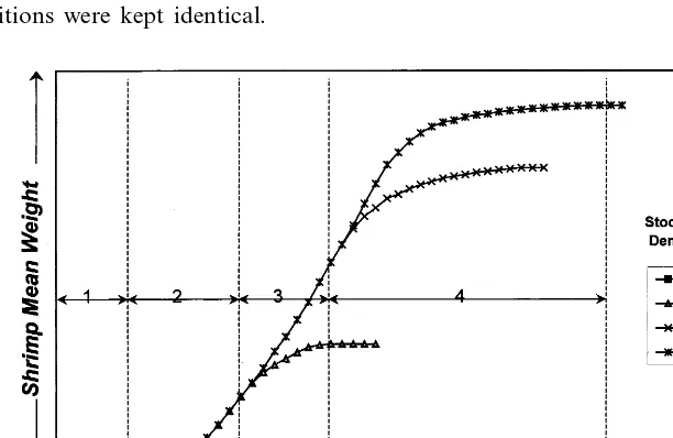
The fact that the shrimp growth rate is approximately inversely proportional to stocking density can be used to optimize the number of stages in a shrimp production system. Fig. 1 shows four idealized stocking-density-dependent growth rate curves. Curve d represents the best growth rate curve, that is to say, the stocking density is set such that at the end of the production period (when the shrimp reach market size), the shrimp continue to maintain their maximum biological growth rate attainable under the environmental and feeding regimes. Curvesa, b and c show that shrimp growth rates are affected by shrimp stocking densities a, b and c, where densities are a\b\c\d. During the beginning of
curvesa, b andc, when the shrimp biomass is below the CSC level, curvesa, b, c
and d are identical. Each growth curve departs from curve d as its CSC level is reached. With an initial stocking density ofa, when the biomass reaches the level represented by CSCa, the biomass in curve a begins to retard the shrimp growth. At
CSCb and CSCc, the shrimp growth rates, as shown by curvesb and cwith initial
maxi-246 J.-K.Wang,J.Leiman/Aquacultural Engineering22 (2000) 243 – 254
mum growth rate that can be attained with the given biological and water management constraints. For a single-stage production system the appropriate stocking density is d.
According to Fig. 1, for a two-stage shrimp production system, we have three choices: either a–d, b–d or c–d. An a–d system will begin with high stocking density a, and at time CSCa the density is reduced to d. For a three-stage
production system, the combinations of a–b–d, a–c–d or b–c–d can be used. There is only one possible design choice for a four-stage production and that is
a–b–c–d.
The number of stages that can be considered in the design process is limited by the available data. As demonstrated by Fig. 1, the four curves,a, b, cand d limit the potential choices to four stages. If more data is available to construct additional growth curves, then the potential number of stages can be correspondingly increased.
In general,
X=2(n−1)
(2)
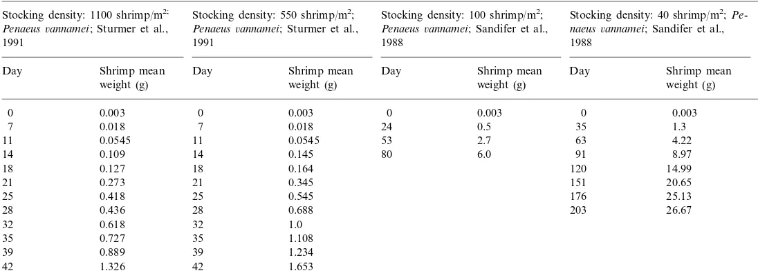
where:Xis number of possible choices in the design of production systems in terms of production stages; n is number of stocking density dependent growth curves. Table 1 gives a summary of all possible configurations using idealized data from Fig. 1. Table 2 shows experimental shrimp growth data from Sturmer et al. (1991), Sandifer et al. (1988). These data give an indication of the effect on shrimp growth rates of stocking densities at 1100, 550, 100, and 40 shrimp/m2 when other conditions were kept identical.
247
Possible phase configurations and corresponding rearing period for CSC theory described in Fig. 3 Staged(days)
Stagea(days) Stageb(days) Stagec(days) Stageadensity Stagebdensity Stagecdensity
Number of Stageddensity
(shrimp/m2)
(shrimp/m2)
(shrimp/m2) (shrimp/m2)
stages
0–21 21–42 42–63 1100 550 100 40
248
Experiment data used to develop the Von Bertallanfy growth curves
Stocking density: 550 shrimp/m2; Stocking density: 100 shrimp/m2;
Stocking density: 1100 shrimp/m2; Stocking density: 40 shrimp/m2;Pe
-Penaeus6annamei; Sturmer et al., Penaeus6annamei; Sturmer et al., Penaeus6annamei; Sandifer et al., naeus6annamei; Sandifer et al.,
1988 1988
1991 1991
Day Shrimp mean Day Shrimp mean
Day Shrimp mean Day Shrimp mean
weight (g)
0.0545 11 0.0545 53 63 4.22
249
J.-K.Wang,J.Leiman/Aquacultural Engineering22 (2000) 243 – 254 Table 3
Von Bertallanfy growth parameters solved by GAMS
Stocking density k(/day) Winf(g) Best-fit line (plot of theoretical equations vs. real R2
data) (shrimp/m2)
1100 0.022 4.1 y=0.0046+0.98x 0.993
y=0.0028+0.95x 0.988
550 0.014 15.0
y=0.22+0.93x 0.993
28.6
100 0.011
y= −0.110+0.97x
40 0.009 44.9 0.993
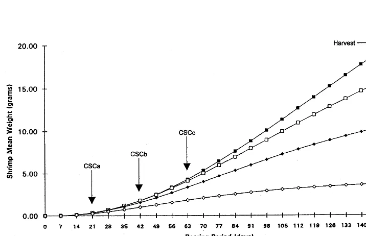
Fig. 2. Shrimp mean weight versus rearing period at various stocking densities.
The Von Bertallanfy equation is one of the best to describe penaeid shrimp growth rates (Tien et al., 1993):
Wt=W*inf[1−e −k*(t-t0)
]n (3)
where: Wt is weight at time t (g); Winf is asymptotic weight (g); t is shrimp age (days);t0 is theoretical age at whichW=0 g (days);kis instantaneous growth rate (g/days); n=2.8025 for Penaeus monodon (Mercy et al., 1993).
The data in Table 2 were compiled using GENERAL ALGEBRAIC MODELING
250 J.-K.Wang,J.Leiman/Aquacultural Engineering22 (2000) 243 – 254
(3). The calculated constants are shown in Table 3 (Leiman, 1995). It can be seen that as stocking densities decrease from 1100 to 40 shrimp/m2, the
k values decrease from 0.022 to 0.009/day, while the Winf values increase from 4.1 to 44.9 g. Using Eq. (3) and the constants from Table 3, we can construct Fig. 2.
While Fig. 1 is an idealized representation, Fig. 2 is based upon limited real data. We can see that Fig. 2 gives an excellent facsimile of Fig. 1.
The total water surface area of the ponds/tanks for each production stage can now be calculated with the following equations and Eq. (1).
I(i)=O(i)/(%S(i))/100 (4)
A(i)=I(i)/SD(i) (5)
where:I(i) is input or stocking population of shrimp in phasei; O(i) is output or transfer/harvest population of shrimp in phase i; %S(i) is % shrimp alive by the end of rearing period in phase i (100% refers to the % shrimp alive at stocking time of phase i); A(i) is water surface area of individual pond/tank in phase i
(m2); SD(i) is stocking density of shrimp in phase i (shrimp/m2).
N(i)=[(tt/h(i)−ts(i))+td(i)]/tpd (6)
where: N(i) is number of ponds/tanks in phase i (integer c); tt/h(i) is transfer/ harvest time in phase i (weeks); ts(i) is stocking time in phase i (weeks); td(i) is down period between cycle in phase i (weeks); tpd is period between product deliveries (weeks)=l/frequency of delivery.
4. Optimization
Setting the market size to be 50 shrimp/kg and the amount of shrimp produced every other week to be 2000 kg of shrimp, Eqs. (4) – (6) are used to calculate the water surface area required. In Eq. (6), N(i) is the number of shrimp tanks and must therefore be an integer; td(i) is the rest period between production cycles used for maintenance and repair and it can be increased so thatN(i) is an integer. It can be seen from Fig. 2 that tanks stocked at initial densities of 1100, 550 and 100 shrimp/m2 will reached their CSC biomass at days 21, 42 and 63, respectively. Shrimp in ponds/tanks stocked at 40 shrimp/m2 grow at the maxi-mum biological growth rate attainable under the environmental and feeding regimes.
251
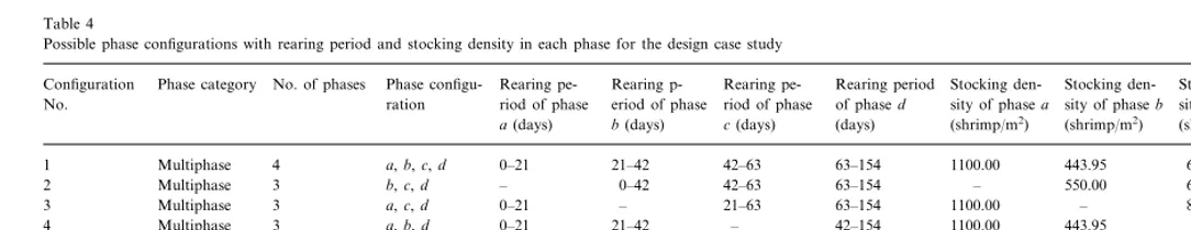
Possible phase configurations with rearing period and stocking density in each phase for the design case study
Phase
configu-Phase category Rearing p- Rearing pe- Rearing period Stocking den- Stocking den- Stocking
den-Configuration No. of phases Rearing pe- Stocking
den-riod of phase eriod of phase sity of phasea
No. ration riod of phase of phased sity of phaseb sity of phasec sity of phased
252 J.-K.Wang,J.Leiman/Aquacultural Engineering22 (2000) 243 – 254
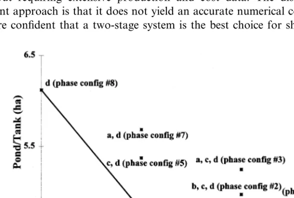
5. Discussion
An analysis was performed to test the sensitivity of the water surface area requirement to changes in CSC values. Every CSC value was first increased by 7 days, so that CSCa, CSCband CSCcvalues were increased to 28, 49, and 70 days,
respectively, and then decreased by 7 days so that CSCa, CSCb and CSCc values
were decreased to 14, 35 and 56 days, respectively. The resultant change in water surface area requirements followed a similar pattern shown in Fig. 3. This relative insensitivity to CSC values indicates to us that the pattern displayed by Fig. 3 is stable and that, in practice, a two-stage production system with a prolonged first stage is optimal for the production of penaeid shrimp. In the present example, the proposed first stage (a prolonged nursery stage) is 42 days.
Based on recent data (1997) from Kona Bay Oyster and Shrimp Company, the final stocking density can probably be raised to 65 shrimp/m2for shrimp averaging 20 – 22 g in weight.
Leiman (1995) developed a procedure to calculate the optimal design of a multi-stage shrimp production system. For those who have data that differs much from the data used in this paper, Leiman’s procedure is available. However, it is our hope that we have shown sufficient evidence that our present conclusion has universal applicability.
The foundation of our analysis is the simplifying assumptions. These assumptions allow us to provide a rough comparison of multi-stage shrimp production systems without requiring extensive production and cost data. The disadvantage of the present approach is that it does not yield an accurate numerical comparison. While we are confident that a two-stage system is the best choice for shrimp production,
253
J.-K.Wang,J.Leiman/Aquacultural Engineering22 (2000) 243 – 254
our present goal is not to produce a two-stage production system design, but merely to show that the two-stage system can be, in most cases, more efficient than either the single-stage or other multi-stage systems. This conclusion, however, is reached without giving due consideration to either the additional stress the shrimp may suffer when transferred from the extended nursery to the grow-out system, or the added management difficulty necessitated by a two-stage system. When extensive comparable biological and financial data become available, our model can be easily modified to yield more accurate comparisons.
References
Brock, J.A., 1992. Current diagnostic methods for agents and diseases of farmed marine shrimp. In: Fulks, W., Main, K.L. (Eds.), Diseases of Cultured Penaeid Shrimp in Asia and the United States. The Oceanic Institute, Honolulu, HI, pp. 209 – 232.
Brooke, A., Kendrick, D., Meeraus, A., 1992. Release 2.25/GAMS/A User’s Guide. The Scientific Press, San Francisco, CA.
Cao, D.G., Jiang, Y., 1990. Origin and nursery of culturedPenaeus chinensisfry. In: Fulks, W., Main, K.L. (Eds.), The Culture of Cold-Tolerant Shrimp: Proceedings of an Asian – U.S. Workshop on Shrimp Culture. The Oceanic Institute, Honolulu, HI, pp. 103 – 109.
Chong, Y.H., 1990. Economic and social considerations for aquaculture site selection: an Asian perspective. In: New, J.B., de Saram, H., Singh, T. (Eds.), Technical and Economic Aspects of Shrimp Farming. Proceedings of the Aquatech ‘90 Conference, 11 – 14 June 1990, Kuala Lumpur, Malaysia, pp. 24 – 36.
Fast, A.W., 1991. Development of appropriate and economically viable shrimp pond growout technol-ogy for the United States. In: DeLoach, P.F., Dougherty, W.J., Davidson, M.A. (Eds.), Frontiers of Shrimp Research. Elsevier, New York, NY, pp. 197 – 240.
Fulks, W., Main, K.L., 1992. Introduction. In: Fulks, W., Main, K.L. (Eds.), Diseases of Cultured Penaeid Shrimp in Asia and the United States. The Oceanic Institute, Honolulu, HI, pp. 3 – 33. LeaMaster, B., 1992. Shrimp health management procedures. In: Fulks, W., Main, K. (Eds.), Diseases
of Cultured Penaeid Shrimp in Asia and the United States. The Oceanic Institute, Honolulu, HI, pp. 345 – 356.
Leiman, J., 1995. Development of a design procedure for multiphase, shrimp grow-out systems. University of Hawaii at Manoa, Honolulu, HI Master of Science Thesis.
Mercy, T.V.A., Koya, M.S.S.I., Vadhyar, K.J., Thampy, D.M., 1993. Length – weight relationship of the pond reared tiger prawnPenaeus monodonfabricius. Fish. Technol. 30 (1), 75 – 76.
Ray, W.M., Chien, Y.H., 1992. Effects of stocking density and aged sediment on tiger prawn,Penaeus monodon, nursery systems. Aquaculture 104 (3/4), 231 – 248.
Samocha, T.M., Lawrence, A.L., 1992. Shrimp nursery systems and management. In: Wyban, J. (Ed.), Proceedings of the Special Session on Shrimp Farming. World Aquaculture Society, Baton Rouge, LA, pp. 87 – 105.
Sandifer, P.A., Hopkins, J.S., Stokes, A.D., 1988. Intensification of shrimp culture in earthen ponds in South Carolina: progress and prospects. J. World Aquac. Soc. 19, 218 – 226.
Sandifer, P.A., Stokes, A.D., Hopkins, J.S., Smiley, R.A., 1991. Further intensification of pond shrimp culture in South Carolina. In: Sandifer, P.A. (Ed.), Shrimp Culture in North America and the Caribbean. World Aquaculture Society, Baton Rouge, LA, pp. 84 – 95.
Stern, S., Letellier, E., 1992. Nursery systems and management in shrimp farming in Latin America. In: Wyban, J. (Ed.), Proceedings of the Special Session on Shrimp Farming. World Aquaculture Society, Baton Rouge, LA, pp. 106 – 109.
254 J.-K.Wang,J.Leiman/Aquacultural Engineering22 (2000) 243 – 254
Tien, S., Leung, P.S., Hochman, E., 1993. Shrimp growth functions and their economic implications. Aquac. Eng. 12, 81 – 96.
Wyban, J., Sweeney, J., 1993. Intensive shrimp production in round ponds. In: McVey, J.P. (Ed.), CRC Handbook of Mariculture. CRC Press, Boca Raton, FL, pp. 275 – 287.