THE GEOMETRIC CORRECTION MODEL BASED ON AREAL FEATURES FOR
MULTISOURCE IMAGES RECTIFICATION
Tengfei LONG, Weili JIAO
Center for Earth Observation and Digital Earth,Chinese Academy of Sciences,No.9 Dengzhuang South Road, Haidian District, Beijing 100094, China - [email protected]
KEY WORDS: Photogrammetry, Rectification, Orientation, Feature, Model, Geometric
ABSTRACT:
The geometric correction model describes the relationship between the features in image and object space. The majority models rely heavily on point-based features to do the rectification. Although it is simple, intuitional and accurate, there are some problems in establishing the accurate model based on point features. In many cases, it is difficult to acquire accurate ground control points in the areas where cross points and corners are not available. On the other hand, image registration based on feature points is greatly confined to the image acquisition time, resolution and spectrum. Due to the above limitations, linear and areal features are used as control features in order to cope with the misidentification problem of points and to register image accurately. This paper proposes a novel geometric correction model based on areal features, which is not confined to a specific imaging geometric model, and can be used for multisource image rectification. The definitions and algorithms of the distance between the areal features and how to establish the error equations using ground control areas (GCAs) are proposed, and geometric correction based on GCAs is achieved. Landsat and ALOS images are used as examples for the test. The experimental results show that the proposed method can be used for different satellite images and imaging models. The correction accuracy when using GCAs is better than one pixel, when the control data does not contain gross errors. The area-based geometric correction model is more fault-tolerant than the point-based model when the control data contains gross errors.
1. INTRODUCTION
Traditional geometric correction model of remote sensing images is based on ground control points (GCPs). When accurate ground control points are available, the point-based geometric correction model can improve the positioning accuracy of the image. However, in the satellite images of some special areas, such as deserts, mountains, it is difficult to identify the accurate point features, therefore sufficient and accurate GCPs are difficult to obtain, while the linear features and areal features (such as roads, water, etc.) are more accessible. On the other hand, when images with different resolutions are taken as reference data, the spatial coordinates of the point cannot be accurately determined. As a matter of fact, it is easier to extract useful areal features than useful point features, and both the natural and human environment is rich in areal features, such as buildings, sports fields, parks and lakes. Moreover, as a lot of areal features appeared in the existing reference images, digital line map (DLG) and GIS vector data, correcting the remote sensing images with areal features can take full advantage of these data.
For a long time, researchers have been focusing on the point-based and line-point-based image registration and geometric correction methods (Habib et al., 2003; Gong et al., 2008; Long et al., 2011a). In recent years, some scholars turn to research on the areal feature based methods from several aspects, including areal feature based image registration (Dare and Dowmanr, 2001; Zhang et al., 2006), areal feature extraction (Zhang and Zhang, 2011; Xin and Zhang, 2011), similarity measure of areal features (Wang, 2008) and areal feature matching strategies (Dong et al., 2007). However, the methods for establishing geometric correction model and performing geometric correction using areal features were rarely involved. At present, the existing methods usually convert the areal features into point features (for example, taking the centre of gravity of the
polygon as the control point (Zhang et al., 2006)), and carry out the geometric correction based on point features. It did not consider the impacts of the sensor imaging method, side angle and topography, which make the areal features in the image deform and make the areal centre of gravity shift.
Starting from the distance measurement of areal features, this paper proposes an area-based geometric correction model for remote sensing image.
2. AREA-BASED GEOMETRIC CORRECTION MODEL
The key technology of the area-based geometric correction model proposed in this paper is to build and solve the error equations using areal features. The establishment of the error equations requires the calculation of distances between polygons, whose prerequisite is the calculation of distances from the points on one polygon to another polygon. Therefore, the following introduces the distance from point to polygon, the distance between polygons and the geometric correction model based on areal features successively.
2.1 Distance from Point to Polygon
The definition of distance from point to polygon is: the distance from point to polygon is the minimum distance from all boundary points of polygon to point , and particularly, the distance is 0 when point is inside of polygon .
The symbol is used to denote the set of all boundary points of polygon , and the distance from point to polygon can be expressed as:
(1) International Archives of the Photogrammetry, Remote Sensing and Spatial Information Sciences, Volume XXXIX-B1, 2012
Where is a boundary point of polygon , is the Euclidean distance between point and point
To get the minimum distance from point to the boundary points of polygon , we need to calculate the distances from point to the edges of polygon first, and then find the minimum distance. There are two cases for the distance from point to an edge of the polygon : construct a perpendicular of segment from point , if the pedal is on segment , the distance from point to edge is the distance from point to the pedal; if the pedal is not on the segment , the distance from point to edge is the smaller one between the distances from point to the two endpoints of segment . The distances from a point to a line segment in different cases are shown in Fig 1. In Fig1(a), the pedal is on the segment , so the distance from point to edge is the length of ; in Fig1(b), the pedal is not on the segment , and , then the distance from point
to segment is the length of .
(a) (b)
Fig1. Distance from point to line segment in two cases. (a) The pedal is on the segment. (b) The pedal is not on the segment.
The distances from a point to a polygon in different cases are shown in Fig 2. In Fig2(a), the pedal of the perpendicular from point to the nearest edge of polygon is on an edge of polygon , so the distance from point to polygon is the length of ; in Fig2(b), the pedal of the perpendicular from point to the nearest edge of polygon is not on an edge of polygon , so the distance from point to polygon is the length of , the distance from point to the nearest vertex of polygon ; in Fig2(c), point is inside of polygon , so the distance from point to polygon is .
(a) (b) (c) Fig2 Distance from point to polygon in different cases. (a) The pedal is on an edge. (b) The pedal is not on an edge. (c) Point is
inside of the polygon.
Considering that adjustment using distance, which is a scalar quantity, is lack of directivity, the definition of distance vector is introduced: if the distance value in formula (1) is obtained
vector from point to polygon , which is denoted as .
Particularly, if , then .
The algorithm for calculating the distance vector from point to polygon is:
Step 1: set as a great value, and is the first edge of polygon ;
Step 2: calculate the distance vector and distance value from point to segment ;
Step 3: if , set , and ;
Step 4: if is the last edge of polygon , turn to Step 5; otherwise, set as the next edge of polygon , and turn to Step 2;
Step 5: output the distance vector from point to polygon .
2.2 Distance between Polygons
Distance between polygons is defined on the basis of distance from point to polygon as: the distance from polygon to polygon is the maximum value of the distances from all boundary points of polygon to polygon .
Particularly, the edge of a polygon is consisted of successive boundary points, while the vertices are the endpoints of polygon. Fig 3 shows the differences between boundary points and vertices of a polygon.
(a) (b)
Fig3. Boundary points and vertices of a polygon: (a) The boundary points of a polygon; (b) The vertices of a polygon. The distance from polygon to polygon can be expressed as:
(2)
Where is a boundary point of polygon
Using this definition to calculate the distance vector between polygons results in large time complexity, and the following proposition may simplify the calculation of the distance vector. Proposition 1: The distance from polygon to polygon is the maximum value of the distances from all vertices of polygon
to polygon .
The proposition 1 can be proved mathematically.
With proposition 1, the vertices set of polygon is denoted as , and the distance from polygon to polygon can be expressed as:
(3) International Archives of the Photogrammetry, Remote Sensing and Spatial Information Sciences, Volume XXXIX-B1, 2012
Where is a vertex of polygon , is an boundary point of polygon
If the distance value from polygon to polygon in formula (3) is obtained when and , the distance vector from polygon to polygon is defined as the vector from point to point , which is denoted as . Particularly, if
, then .
The algorithm for calculating the distance vector from polygon to polygon is:
Step 1: set , and is the first vertex of polygon ; Step 2: calculate the distance vector and distance value from point to polygon ;
Step 3: if , set and ;
Step 4: if is the last vertex of polygon , turn to Step 5; otherwise, set as the next vertex of polygon , and turn to Step 2;
Step 5: output the distance vector from polygon to polygon .
2.3 Establishment of Area-based Geometric Correction Model
The classic imaging model used to create the relationship between the three-dimensional spatial coordinate of ground point and plane coordinates of the corresponding image point, and in general, the generic model can be expressed as formula (4).
(4)
where denotes the parameters of geometric correction model of the sensor
denotes the spatial coordinates of the ground control points (GCPs)
is a boundary point of polygon
denotes the coordinates of GCPs in image plane
At present, the commonly used geometric correction models include strict imaging model, affine model, polynomial model, Rational Function Model (RFM), and etc. All these models can be expressed as formula (4) (Long et al., 2011b), and the method proposed in this paper can be used for a variety of geometric correction models. The following describes the process of establishing the error equations using areal features.
Areal features are usually denoted as polygons. A ground control area (GCA) is consisted of a ground polygon and an image polygon . The polygon is consisted of vertices, whose coordinates are . The polygon is consisted of vertices, whose coordinates are . The projection polygon of the ground polygon in image can be calculated according to formula (4), and the vertices of is denoted as , and the following constrain between polygon and polygon should be met:
(5)
Formula (5) indicates that the distance vector from polygon to polygon is . According to the formula (3), the distance from polygon to polygon should be obtained at some vertex of polygon , and suppose it is , where is an integer between and , then:
(6)
where polygon is a known quantity
has two components in horizontal and vertical direction, and can be denoted as
The following formula is according to formula (4):
(7)
where is the vertex of the ground polygon . Then the formula (6) is equivalent to formula (8).
(8)
Error equations of GCAs can be established by linearizing the formula (8):
(9)
where and are random errors
denotes the correction vector of
Considering that there is no analytical form for and , the approach of numerical differentiation (Burden and Faires, 2011) is used to approximate the partial derivatives of each function, such as:
(10)
As two error equations such as formula (9) can be derived from a GCA, the unknown parameters of the model can be solved by using no less than GCAs, and the LM algorithm (More, 1977) may be applied to calculation of the parameters.
3. TEST AND RESULT ANALYSIS
In order to verify the validity of the proposed method, a Landsat TM image and an ALOS PRISM image are used in the tests. The Landsat image was taken in April 2008 in Anhui province, and the image size is 6856 pixels×5733 pixels, and the spatial resolution is 30 meters. The ALOS image was taken in September 2010 in Jilin province, and the image size is 29493 pixels×16000 pixels, while the spatial resolution is 2.5 meters. Both of the maximum elevation differences of the area covered by the two images are less than 400 meters.
Four tests are carried out for both TM and ALOS images. In the first test, several evenly distributed GCAs are used for the geometric correction. In the second test, a pair of corresponding vertices is selected from each GCA in the first test, and then all these pairs of points are used as GCPs for the geometric
correction. Two gross errors (5~6 pixels) are artificially added in the GCPs and GCAs of the first and second test, and the errors added in the GCPs are the same as those added in the GCAs. In the third test, the GCAs with gross errors are used for geometric correction. In the fourth test, the GCPs with gross errors are used for the geometric correction. The same check points (CPs) are used to evaluate the accuracy of the result in all the tests. The correction of Landsat image is based on the satellite orbital model (Chen et al., 2009), and the correction of ALOS image is based on the RFM with image compensation (Grodecki and Dial, 2003). The experimental results of the two images are shown in Table 1, including the fitting accuracy of the GCAs, the fitting accuracy of the GCPs, and the accuracy of the check points.
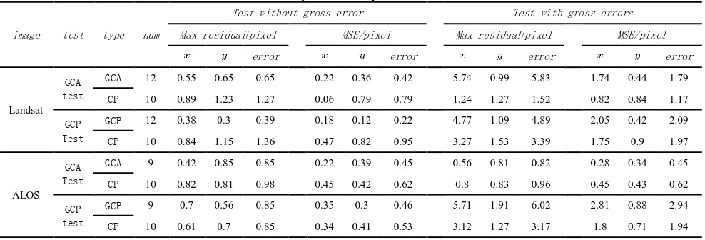
Table 1 Comparison of experimental results
image test type num
Test without gross error Test with gross errors
Max residual/pixel MSE/pixel Max residual/pixel MSE/pixel
error error error error
(1) The proposed area-based geometric correction method can be applied to different satellite images and different imaging models.
(2) When the control data does not contain gross errors, the image correction using geometric correction model based on GCAs gains almost the same accuracy as that based on GCPs. As shown in Table 1, in the tests of Landsat and ALOS image without gross errors, the errors of the check points when using GCPs and using GCAs can both be less than one pixel.
(3) When the control data contains gross errors, the geometric correction model based on GCAs is more fault-tolerant than the geometric correction model based on GCPs. As shown in Table 1, in the tests of Landsat image with gross errors, the maximum residual of check points is more than 3 pixels when the GCPs are used for geometric correction, while the maximum residual of check points is less than 2 pixels when the GCAs are used for geometric correction. In the test of ALOS image with gross errors, the maximum residual of check points is more than 3 pixels when the GCPs are used for geometric correction, while the maximum residual of check points is less than 1 pixel when the GCAs are used for geometric correction. In the GCAs test of Landsat image with gross errors, the gross errors which involved in the calculation of the model may result in the
therefore the impact of this gross error on the accuracy of the area-based geometric correction model is limited. In the GCAs test of ALOS image with gross errors, as the gross error points are inside of the reference area features, and the distances from those points to the reference polygons is , the gross error features in the reference images, the digital line maps, and GIS vector data, the use of areal features in geometric correction may take full advantage of the data. On the other hand, since an areal feature is consisted of many points, gross errors in individual points do not remarkably reduce the accuracy of the areal feature, therefore the geometric correction model based on GCAs is more fault-tolerant than the geometric correction model based on GCPs. The results of the tests show that the method proposed in this paper can be used for different satellite images and imaging models. When the control data does not
Burden, R.L. and Faires, J.D., 2011. Numerical analysis. (Ninth International Archives of the Photogrammetry, Remote Sensing and Spatial Information Sciences, Volume XXXIX-B1, 2012
Chen, P.S.; Jiao, W.L.; Jia, X.P.; Wang, W., 2009. Robust LM Algorithm and Its Application on Rigorous Physical Model. Science Technology and Engineering, 9(16), pp. 4614-4618. Dare, P. and Dowmanr, I., 2001. An improved model for automatic feature-based registration of SAR and SPOT image. ISPRS Journal of Photogrammetry & Remote Sensing, 56(1), pp. 13-28.
Dong, X.H.; Deng, S.S.; Shi, W.Z., 2007. A Probabilistic Theory-based Matching Method. ACTA GEODAETICA et CARTOGRAPHICA SINICA, 36(2), pp. 210-217.
Gong, D.C.; Tang, X.T.; Li, S.Z.; Hu, G.J., 2008. Image Registration of High Resolution Remote Sensing Based on Straight-line Feature. The International Archives of the Photogrammetry, Remote Sensing and Spatial Information Sciences. Vol. XXXVII. Part B4. pp. 1819-1823.
Grodecki, J. and Dial, G., 2003. Block Adjustment of High-Resolution Satellite Images Described by Rational Polynomials, Photogrammetric Engineering & Remote Sensing, 69(1), pp. 59-68.
Habib, A.F.; Lin, H.T.; and Morgan, M., 2003. Autonomous space resection using point- and line-based representation of free-form control linear features, The Photogrammetric Record, 18(103), pp. 244–258.
Long, T.F.; Jiao, W.L.; Wang, W., 2011a. Geometric Rectification Using Feature Points Supplied by Straight-lines. Procedia Environmental Sciences, 11 (2011), pp. 200-207. Long, T.F.; Jiao, W.L.; Wang, W., 2011b. Block Adjustment for Generic Geometric Model Using Points and Straight-Lines. Advanced Materials Research, Vols. 268-270(2011), pp. 584-589.
More, J.J., 1997. The Levenberg-Marquardt algorithm: implementation and theory, in: G.A. Watson, ed., Numerical Analysis Dundee 1977, Lecture Notes in Mathematics 630 (Springer-Verlag, Berlin, 1977) pp. 105-116.
Wang, X., 2008. Research on Identical Entity Geometric Matching in Multi-Source Spatial Data. Zhengzhou:PLA Information Engineering University.
Xin, L. and Zhang, J.X., 2011. Fast Extraction of Conjugated Area Features and Accurate Registration of Remote Sensing Image. Geomatics and Information Science of Wuhan University, 36(6), pp. 678-682.
Zhang, X.D.; Li, D.R.; Gong, J.Y., Qin, Q.Q., 2006. A Matching Method of Remote Sensing Image and GIS Data Based on Area Feature. JOURNAL OF REMOTE SENSING, 10(3), pp. 373-380.
Zhang, Y. and Zhang, J.X., 2011. Edge Detection and Areal Feature Extraction Based on Improved LOG Operator. Journal of Geomatics, 36(5), pp. 8-10.
Acknowledgements
The research has been supported by the National High Technology Research and Development Program of China (863 Program) under grant number 2006AA12Z118 and 2012BAH27B05.