This content has been downloaded from IOPscience. Please scroll down to see the full text.
Download details:
IP Address: 202.94.83.84
This content was downloaded on 10/03/2016 at 00:16
Please note that terms and conditions apply.
View the table of contents for this issue, or go to the journal homepage for more
A modified Mohapatra–Chaudhry two-four finite
difference scheme for the shallow water equations
L K Budiasih1,2,3, L H Wiryanto2, and S Mungkasi1 1
Department of Mathematics, Faculty of Science and Technology, Sanata Dharma University, Mrican, Tromol Pos 29, Yogyakarta 55002, Indonesia
2
Department of Mathematics, Faculty of Mathematics and Natural Sciences, Bandung Institute of Technology, Jalan Ganesha 10, Bandung 40132, Indonesia
E-mail: lusia [email protected], [email protected], [email protected]
Abstract. A two-four finite difference scheme for Boussinesq equations was developed by Mohapatra and Chaudhry in 2004. This scheme is of course also applicable to solve the shallow water equations. However this scheme is not robust to deal with dry bed, that is, spurious oscillations appear around wet-dry areas. In this paper we propose a modified two-four finite difference scheme to solve the shallow water equations involving (almost) dry bed. The modified scheme has fewer number of divisions by zero or almost zero, and at the same time, only conserved quantities (mass and momentum) are used in the evolution of the new scheme. The modification lies on the discretisation of the momentum equation. We discretise the momentum equation using the momentum variable itself rather than using the velocity variable as done by Mohapatra and Chaudhry. Numerical results show that our proposed scheme is more robust for wetting and drying processes of the shallow water equations.
1. Introduction
Shallow water flows can be described using a mathematical model, such as the system of either shallow water equations or Boussinesq equations. These equations have been used to simulate river flows, floods, and even tsunamis. Therefore, accurately solving these equations is very important.
Mohapatra and Chaudhry [6] simulated dam-break flows numerically by solving the one-dimensional Boussinesq equations using a two-four explicit finite-difference scheme. Readers interested in the analytical study of the Mohapatra–Chaudhry scheme are referred to [6] and references therein. The Mohapatra–Chaudhry scheme was validated by comparing the computed results with the Stoker solution [13, 14], yielded satisfactory results for dam-break flow studies. Their numerical tests were based on a wet bed assumption, in which the upstream and downstream positions are wet. However, in actual flow situation, there is another problem, known as a dry bed problem, in which the downstream depth is close to or absolutely zero. The Mohapatra–Chaudhry scheme is not robust to deal with dry bed, because the scheme produces spurious oscillations around wet-dry areas.
When solving the dry bed problem, numerical schemes usually face extra challenges. Supercritical and subcritical flows may coexist for flow in horizontal [1, 2, 4]. A difficulty in
3
L K Budiasih is a mathematics lecturer at Sanata Dharma University and currently a Ph.D. student at the Department of Mathematics, Faculty of Mathematics and Natural Sciences, Bandung Institute of Technology.
dealing with simulation of dam-break flows on a dry bed lies in the downstream boundary conditions of the flow field, where the flow depth goes to zero [15]. There may also be discontinuity in the velocity at the wet-dry interface, whereas the depth and momentum values are continuous.
To overcome the wet-dry problem, in this paper we propose a modified Mohapatra–Chaudhry scheme, in which only conserved quantities (mass and momentum) are used in the evolution of the new scheme, to solve the shallow water equations. Numerical results show that our proposed scheme performs better for wetting and drying processes of the shallow water equations than the original Mohapatra–Chaudhry scheme.
2. Governing equations
Consider one-dimensional shallow water equations, which are written as continuity and momentum equations [6]:
where x denotes the longitudinal direction; u represents the depth-averaged velocity in the x -direction; tis the time variable; h denotes the flow depth; g represents the acceleration due to gravity; S0 is the bed slope in the x-direction; and Sf is the friction slope in the x-direction.
The friction slope, Sf, is calculated from the Manning equation
Sf = u2n2
h4/3 (3)
with n is the Manning roughness coefficient and the channel is assumed to be wide and rectangular. A simplification and an extension of the one-dimensional shallow water equations were discussed in some literatures, such as Mungkasi and Roberts [8, 9, 11, 12].
The derivation of the above equations is based on assumption that the velocity in the vertical direction varies linearly from zero at the bed to the maximum value at the surface. The governing equations do not account for the effective stresses arising due to laminar viscous stresses, turbulence stresses and stresses due to depth averaging. Note that the shallow water equations are special cases of the Boussinesq equations with the values of Boussinesq terms are zero.
3. Numerical model
There are mathematical and physical reasons why the Mohapatra–Chaudhry scheme needs modification for dry bed involvement in solving the shallow water equations. Mathematically, the Mohapatra–Chaudhry scheme has two divisions by zero or almost zero number for calculating the velocity. That is, one division occurs in the predictor step and another one in the corrector step. These divisions make the computation results tend to large numbers, and hence, give large errors. Physically, evolving the velocity in the predictor and corrector steps is not the best option when there exists discontinuity in the solution, because velocity is not a conserved quantity.
Therefore, we propose a modified scheme having fewer number of divisions by zero or almost zero, and at the same time, only conserved quantities (mass and momentum) are used in the evolution of the new scheme. Similar to the Mohapatra–Chaudhry scheme, the governing equations (Eqs. (1) and (2)) are solved using a two-four finite difference scheme on collocated grids. However in the modified scheme, the momentum equation in Eq. (2) is discretised using the momentum variable q = uh. For each iteration, variables hk+1 and (uh)k+1 at an
unknown time t+ ∆tare computed explicitly from variables hk and (uh)k at the known time t
in three phases. First, a predictor procedure yields predicted variables hp and (uh)p. Second,
a corrector procedure produces corrected variables hc and (uh)c. Third, the flow field (˜h,uh˜) is then computed by taking the average of the variables at the known time level, k, and the corrector part. The solution of the third phase will be the final approximate solution at time
t+ ∆t.
3.1. Predictor part
The predicted water level variable is the same as in the Mohapatra–Chaudhry scheme. It is obtained from the known variables by using the forward finite differencing for both the time and space derivatives, as follows
The equation to compute the predicted velocity variable in the Mohapatra–Chaudhry scheme is modified to obtain the predicted momentum variable:
(uh)pi = (uh)ki +1
Notice that in this predicted part we evaluate the predicted momentum variable directly, without computing the predicted velocity variable.
3.2. Corrector part
The corrected water level variable in the modified scheme is obtained from the predicted variables by using the forward finite differencing for the time derivatives and backward finite differencing for the space derivatives, as in the Mohapatra–Chaudhry scheme:
hci =hpi +1
As in the predictor part, the equation to compute the corrected velocity variable in the Mohapatra–Chaudry scheme is modified to obtain the corrected momentum variable:
(uh)ci = (uh)pi +1
As in the predicted part, the corrector velocity variable is not evaluated in this corrector part. The solutions of the predictor-corrector procedure in the modified scheme are the values of water depth and momentum.
3.3. Final step
Flow variables (˜h,uh˜ ) are then evaluated by taking the average of variable values at the known time level kand the corrector part:
In case the velocity values are desired, it can be computed as
˜
ui =
˜ (uh)i
˜
hi
. (11)
The values of water depth and momentum at the end of each time step are smoothened by utilising the artificial viscosity procedure [5]. The smoothened values are then used for the next interation. Note that the artificial viscosity procedure is used in order to be consistent with Mohapatra–Chaudhry’s paper. By numerical experiments we have found that the artificial viscosity procedure stabilises the solution near vacuum.
3.4. Initial and boundary conditions
As the modified scheme uses the variables h and q = uh for discretisation, it is necessary to adjust the initial and boundary conditions of the variables, as follows:
The inital condition, att= 0.0, is given
hi=hu for i≤idam, (12)
hi =hd for i > idam, (13)
(uh)i= 0.0 for all i, (14)
and the boundary condition, att >0.0, is given
h1 =h2=h3 =hu, (15)
hilast =hilast−1 =hilast−2=hd, (16)
(uh)1= (uh)2 = (uh)3 = 0.0, (17)
(uh)ilast = (uh)ilast−1 = (uh)ilast−2= 0.0. (18)
The time step ∆t is computed using the stability condition governed by the Courant– Friedrichs–Lewy (CFL) condition. The necessary condition for stability of the two-four scheme is that:
∆t=Cn
∆x
max(|u|+√gh), (19) where Cn ≤ 2/3, is satisfied [3]. Here Cn is the Courant number, which is also known as the
CFL number.
4. Results
In this section, the modified scheme is used to solve the shallow water equations to simulate dam-break flows on wet and dry bed, with flat bottom without friction. The problem is set by equations (1) and (2), where the bed slopeS0 = 0.0, and the friction slopeSf = 0.0, with initial
conditions
u(x,0) = 0 and h(x,0) =
(
hu if x < x0 hd if x > x0
(20)
both hu and hd are nonnegative and hu > hd. At time t = 0, the dam wall is immediately
removed and the water on upstream flows to the downstream at the subsequent time t, as illustrated in Figure 1.
The modified scheme is validated by comparing its results with those of the Mopatra-Chaudhry scheme and the analytical solution to the shallow water equations (see [7, 10, 13, 14]
Dam Water surface at time t = 0
Water surface at time t > 0
Figure 1. Schematic illustration of the solution to the dam-break problem with a finite water depth downstream at timet >0
0 5 10 15 20 25 30 35 40 45 50
0 0.5 1
Water surface at time t=5.000
analytical solution modified scheme Mohapatra−Chaudhry
0 5 10 15 20 25 30 35 40 45 50
0 0.5 1
Water velocity at time t=5.000
analytical solution modified scheme Mohapatra−Chaudhry
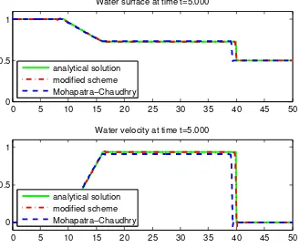
Figure 2. Water profile of dam-break on a wet bed at t= 5, with hu = 1.0 and hd= 0.5
for derivation of the analytical solution). For this purpose, the following input parameters are used: channel length, L = 50.0; dam location, Ld = 25.0; initial velocity is zero; acceleration
due to gravity, g= 9.8; Manning roughness coefficient,n= 0; Courant number,Cn= 0.6.
For the dam-break problem over wet bed, we consider two cases: dam with the initial water depth in the upstream, hu = 1.0, the initial downstream level are hd = 0.5 and hd = 0.2
0 5 10 15 20 25 30 35 40 45 50 0
0.5 1
Water surface at time t=5.000
analytical solution modified scheme Mohapatra−Chaudhry
0 5 10 15 20 25 30 35 40 45 50
0 0.5 1 1.5 2
Water velocity at time t=5.000
analytical solution modified scheme Mohapatra−Chaudhry
Figure 3. Water profile of dam-break on a wet bed at t= 5, with hu = 1.0 and hd= 0.2
0 5 10 15 20 25 30 35 40 45 50
0 0.5 1
Water surface at time t=1.000
analytical solution modified scheme Mohapatra−Chaudhry
0 5 10 15 20 25 30 35 40 45 50
−5 0 5
Water velocity at time t=1.000
analytical solution modified scheme Mohapatra−Chaudhry
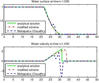
Figure 4. Water profile of dam-break on a dry bed att= 1, withhu= 1.0 and hd= 10−9
In case the initial downstream level is zero (almost zero), that is a dry bed problem (almost dry), in this simulation we considerhd= 10−9. Figure 4 ilustrates the water profile att= 1 after
the dam destruction. This shows that the modified scheme is more robust for wetting process of the shallow water equations. If we simulate for a large time value, the Mohapatra–Chaudhry scheme is unstable even though the CFL condition is satisfied. Note that the CFL condition is a necessary condition for stability, and not the sufficient condition.
5. Conclusions
A modified two-four finite difference scheme is utilised to solve the shallow water equations for simulating dam-break flows over wet and dry bed. We modify the discretisation of the momentum equation from using the velocity variable, as done by Mohapatra and Chaudhry, to using the momentum variable itself. Numerical results show that the scheme is more accurate for wetting process of the shallow water equations. This suggests that the scheme is also robust for wetting and drying processes.
6. References
[1] Chaudhry M H 2008Open Channel Flow(Springer, New York)
[2] Chen C 2006 High order shock capturing schemes for hyperbolic conservation laws and the application in open channel flowsPhD Thesis(University of Kentucky, Lexington)
[3] Gharangik A M and Chaudhry M H 1991 Numerical simulation of hydraulic jump Journal of Hydraulic Engineering1171195-1211
[4] Henderson F M 1966Open Channel Flow(Macmillan, New York)
[5] Jameson A, Schmidt W and Turkel E 1981 Numerical solutions of the Euler equations by finite volume methods using Runge-Kutta time stepping schemes AIAA 14th Fluid and Plasma Dynamic Conference
Paper 1981-12591-17
[6] Mohapatra P K and Chaudhry M H 2004 Numerical solution of Boussinesq equations to simulate dam-break flowsJournal of Hydraulic Engineering130156-159
[7] Mungkasi S and Roberts S G 2010 A new analytical solution for testing debris avalanche numerical models
ANZIAM Journal52C349-C363
[8] Mungkasi S and Roberts S G 2010 Numerical entropy production for shallow water flowsANZIAM Journal
52C1-C17
[9] Mungkasi S and Roberts S G 2011 A finite volume method for shallow water flows on triangular computational grids Proceedings of The 2011 IEEE International Conference on Advanced Computer Science and Information System(ICACSIS 2011)79-84
[10] Mungkasi S and Roberts S G 2012 Analytical solutions involving shock waves for testing debris avalanche numerical modelsPure and Applied Geophysics1691847-1858
[11] Mungkasi S and Roberts S G 2012 Approximations of the Carrier-Greenspan periodic solution to the shallow water wave equations for flows on a sloping beachInternational Journal for Numerical Methods in Fluids
69763-780
[12] Mungkasi S and Roberts S G 2013 Validation of ANUGA hydraulic model using exact solutions to shallow water wave problemsJournal of Physics: Conference Series423012029
[13] Stoker J J 1948 The formation of breakers and bores the theory of nonlinear wave propagation in shallow water and open channelsCommunications on Pure and Applied Mathematics11-87
[14] Stoker J J 1957 Water Waves: The Mathematical Theory with Application (Interscience Publishers, New York)
![[Modul Konsep Jaringan] BAB 1 Pengenalan Jaringan Komputer](data:image/gif;base64,R0lGODlhAQABAIAAAP///wAAACH5BAEAAAAALAAAAAABAAEAAAICRAEAOw==)