El e c t ro n ic
Jo ur
n a l o
f P
r o
b a b il i t y
Vol. 15 (2010), Paper no. 27, pages 801–894. Journal URL
http://www.math.washington.edu/~ejpecp/
Convergence of the critical finite-range contact process to
super-Brownian motion above the upper critical
dimension:
The higher-point functions
Remco van der Hofstad
∗Akira Sakai
†Abstract
We consider the critical spread-out contact process inZd withd≥1, whose infection range is denoted by L ≥ 1. In this paper, we investigate the higher-point functionsτ(r)
~t (~x)for r ≥3, whereτ(r)
~t (~x)is the probability that, for alli=1, . . . ,r−1, the individual located atxi ∈Z d is infected at timetiby the individual at the origino∈Zdat time 0. Together with the results of the 2-point function in[16], on which our proofs crucially rely, we prove that ther-point functions converge to the moment measures of the canonical measure of super-Brownian motion above the upper critical dimension 4. We also prove partial results for d ≤ 4 in a local mean-field setting.
The proof is based on the lace expansion for the time-discretized contact process, which is a version of oriented percolation inZd×ǫZ
+, where ǫ ∈ (0, 1] is the time unit. For ordinary
oriented percolation (i.e., ǫ = 1), we thus reprove the results of [20]. The lace expansion coefficients are shown to obey bounds uniformly inǫ∈(0, 1], which allows us to establish the scaling results also for the contact process (i.e., ǫ ↓0). We also show that the main term of the vertex factor V, which is one of the non-universal constants in the scaling limit, is 2−ǫ
(=1 for oriented percolation,=2 for the contact process), while the main terms of the other non-universal constants are independent ofǫ.
∗Department of Mathematics and Computer Science, Eindhoven University of Technology, 5600 MB Eindhoven, The
The lace expansion we develop in this paper is adapted to both the r-point function and the survival probability. This unified approach makes it easier to relate the expansion coefficients derived in this paper and the expansion coefficients for the survival probability, which will be investigated in[18].
Key words:contact process, mean-field behavior, critical exponents, super-Brownian motion. AMS 2000 Subject Classification:Primary 60J65.
1
Introduction and results
1.1
Introduction
The contact process is a model for the spread of an infection among individuals in thed-dimensional integer lattice Zd. Suppose that the origin o ∈ Zd is the only infected individual at time 0, and
assume for now that every infected individual may infect a healthy individual at a distance less than
L ≥ 1. We refer to this type of model as the spread-out contact process. The rate of infection is denoted byλ, and it is well known that there is a phase transition inλat a critical valueλc∈(0,∞)
(see, e.g.,[24]).
In the previous paper[16], and following the idea of [25], we proved the 2-point function results for the contact process for d >4 via a time discretization, as well as a partial extension to d ≤4. The discretized contact process is a version of oriented percolation inZd×ǫZ+, whereǫ∈(0, 1]is
the time unit andZ+is the set of nonnegative integers: Z+={0}∪˙ N. The proof is based on the
strategy for ordinary oriented percolation (ǫ=1), i.e., on the application of the lace expansion and an adaptation of the inductive method so as to deal with the time discretization.
In this paper, we use the 2-point function results in[16]as a key ingredient to show that, for any
r≥3, the r-point functions of the critical contact process ford>4 converge to those of the canon-ical measure of super-Brownian motion, as was proved in[20]for ordinary oriented percolation. We follow the strategy in[20]to analyze the lace expansion, but derive an expansion which is dif-ferent from the expansion used in [20]. The lace expansion used in this paper is closely related to the expansion in[15] for the oriented-percolation survival probability. The latter was used in
[14]to show that the probability that the oriented-percolation cluster survives up to timendecays proportionally to 1/n. Due to this close relation, we can reprove an identity relating the constants arising in the scaling limit of the 3-point function and the survival probability, as was stated in[13, Theorem 1.5]for oriented percolation.
The main selling points of this paper in comparison to other papers on the topic are the following:
1. Our proof yields a simplification of the expansion argument, which is still inherently difficult, but has been simplified as much as possible, making use of and extending the combined insights of[9; 15; 16; 20].
2. The expansion for the higher-point functions yields similar expansion coefficients to those for the survival probability in[15], thus making the investigation of the contact-process survival probability more efficient and allowing for a direct comparison of the various constants arising in the 2- and 3-point functions and the survival probability. This was proved for oriented percolation in [13, Theorem 1.5], which, on the basis of the expansion in [19], was not
directly possible.
3. The extension of the results to certain local mean-field limit type results in low dimensions, as was initiated in[5]and taken up again in[16].
The investigation of the contact-process survival probability is deferred to the sequel [18] to this paper, in which we also discuss the implications of our results for the convergence of the critical spread-out contact process towards super-Brownian motion, in the sense of convergence of finite-dimensional distributions[23]. See also[12]and[28]for more expository discussions of the var-ious results for oriented percolation and the contact process for d > 4, and [29] for a detailed discussion of the applications of the lace expansion. For a summary of all the notation used in this paper, we refer the reader to the glossary in Appendix A at the end of the paper.
1.2
Main results
We define the spread-out contact process as follows. LetCt⊆Zdbe the set of infected individuals at
timet ∈R+≡[0,∞), and letC0={o}. An infected sitex recovers in a small time interval[t,t+ǫ]
with probabilityǫ+o(ǫ)independently oft, whereo(ǫ)is a function that satisfies limǫ↓0o(ǫ)/ǫ=0. In other words, x ∈Ct recovers at rate 1. A healthy site x gets infected, depending on the status
of its neighboring sites, at rateλPy∈C
tD(x− y), whereλ≥0 is the infection rate. We denote the associated probability measure byPλ. We assume that the function D:Zd →[0, 1]is a probability distribution which is symmetric with respect to the lattice symmetries. Further assumptions on D
involve a parameterL≥1 which serves to spread out the infections, and will be taken to be large. In particular, we require that D(o) =0 and kDk∞≡supx∈ZdD(x)≤C L−d. Moreover, withσdefined as
σ2=X
x
|x|2D(x), (1.1)
where| · |denotes the Euclidean norm onRd, we require thatC1L≤σ≤C2Land that there exists
a∆>0 such that X
x
|x|2+2∆D(x)≤C L2+2∆. (1.2)
See[16, Section 5]for the precise assumptions onD. A simple example ofDis
D(x) =
1{0<kxk∞≤L}
(2L+1)d−1, (1.3)
which is the uniform distribution on the cube of radius L.
Forr≥2,~t= (t1, . . . ,tr−1)∈Rr+−1and~x= (x1, . . . ,xr−1)∈Z(r−1)d, we define the r-point function as
τ~λt(~x) =Pλ(xi ∈Ct
i ∀i=1, . . . ,r−1). (1.4) For a summable function f:Zd
→R, we define its Fourier transform fork∈[−π,π]d by ˆ
f(k) = X
x∈Zd
eik·xf(x). (1.5)
By the results in[8]and the extension of[2]to the spread-out model, there exists a unique critical pointλc∈(0,∞)such that
Z ∞
0
dt τˆλt(0)
(
<∞, ifλ < λc,
=∞, otherwise, limt↑∞P
λ(C
t6=∅)
(
=0, ifλ≤λc,
>0, otherwise. (1.6)
We will next investigate the sufficiently spread-out contact process at the critical valueλcford>4,
1.3
Previous results for the 2-point function
We first state the results for the 2-point function proved in[16]. Those results will be crucial for the current paper. In the statements,σis defined in (1.1) and∆in (1.2).
Besides the high-dimensional setting for d > 4, we also consider a low-dimensional setting, i.e.,
d≤4. In this case, the contact process isnotbelieved to be in the mean-field regime, and Gaussian asymptotics are thus not expected to hold as long as L remains finite. However, inspired by the mean-field limit in [5] of Durrett and Perkins, we have proved Gaussian asymptotics when range and time grow simultaneously[16]. We suppose that the infection range grows as
LT=L1Tb, (1.7)
where L1≥1 is the initial infection range and T ≥1. We denote byσ2T the variance of D=DT in this situation. We will assume that
α=bd+d−4
2 >0. (1.8)
Theorem 1.1(Gaussian asymptotics for the two-point function). (i) Let d>4,δ∈(0, 1∧∆∧
d−4
2 )and L ≫1. There exist positive finite constants A=A(d,L), v = v(d,L)and Ci = Ci(d)
(i=1, 2) such that
ˆ
τλc
t pk vσ2t
=A e−|k|
2 2d
1+O |k|2(1+t)−δ+O (1+t)−(d−4)/2, (1.9) 1
ˆ
τλc
t (0)
X
x
|x|2τλc
t (x) =vσ2t
1+O (1+t)−δ, (1.10)
C1L−d(1+t)−d/2≤ kτλc
t k∞≤e−
t+C
2L−d(1+t)−d/2, (1.11)
with the error estimate in(1.9)uniform in k∈Rd with
|k|2/log(2+t)sufficiently small. More-over,
λc=1+O(L−d), A=1+O(L−d), v=1+O(L−d). (1.12)
(ii) Let d≤4,δ∈(0, 1∧∆∧α)and L1 ≫1. There existλT =1+O(T−µ)for someµ∈(0,α−δ)
and Ci=Ci(d)(i=1, 2) such that, for every0<t≤logT ,
ˆ
τλT
T t k
p σ2
TT t
=e−|k|
2 2d
1+O(T−µ) +O |k|2(1+T t)−δ, (1.13) 1
ˆ
τλT
T t(0)
X
x
|x|2τλT
T t(x) =σ
2
TT t
1+O(T−µ) +O (1+T t)−δ, (1.14)
C1L−Td(1+T t) −d/2
≤ kτλT
T tk∞≤e−
T t+C
2L−Td(1+T t)
−d/2, (1.15)
with the error estimate in(1.13)uniform in k∈Rd with|k|2/log(2+T t)sufficiently small.
In the rest of the paper, we will always work at the critical value, i.e., we takeλ = λc for d >4
and λ = λT as in Theorem 1.1(ii) for d ≤ 4. We will often omit the λ-dependence and write
τ(r)
~t (~x) =τ
λ
~t(~x)to emphasize the number of arguments ofτ
Whileτλc
t (x)tells us what paths in a critical cluster look like,τ
λc
~t (~x)gives us information about the
branching structure of critical clusters. The goal of this paper is to prove that the suitably scaled critical r-point functions converge to those of the canonical measure of super-Brownian motion (SBM).
In [5], Durrett and Perkins proved convergence to SBM of the rescaled contact process with LT defined in (1.7). We now compare the ranges needed in our results and in [5]. We need that
α≡ bd+d−24 >0, i.e., bd> 4−2d. In[5], bd =1 for alld≥3, and L2T ∝TlogT ford =2, which is the critical case in[5]. In comparison, we are allowed to use ranges that grow to infinity slower than the ranges in[5]whend≥3, but the range ford=2 in our results needs to be slightly larger than the range in[5]. It would be of interest to investigate whether a range L2T ∝ TlogT or even smaller is possible by adapting our proofs.
1.4
The
r
-point function for
r
≥
3
To state the result for ther-point function forr ≥3, we begin by describing the Fourier transforms of the moment measures of SBM. These are most easily defined recursively, and will serve as the limits of ther-point functions. We define
ˆ
M(1)
t (k) =e−
|k|2
2dt, k∈Rd, t∈R+, (1.16)
and define recursively, forr≥3,
ˆ
M(r−1)
~t (~k) =
Z t
0
dtMˆ(1)
t (k1+· · ·+kl)
X
I⊂J1:|I|≥1 ˆ
M~t(|I|)
I−t(~kI) ˆM
(l−|I|)
~tJ\I−t(
~kJ\I), ~k∈Rd l,~t
∈Rl+, (1.17)
where J ={1, . . . ,r−1}, J1 =J\ {1}, t =miniti,~tI is the vector consisting of ti withi∈I, and
~tI−t is subtraction of t from each component of~tI. The quantity Mˆ(l)
~t (~k) is the Fourier transform
of the lth moment measure of the canonical measure of SBM (see [20, Sections 1.2.3 and 2.3]for more details on the moment measures of SBM).
The following is the result for the r-point function for r≥3 linking the critical contact process and the canonical measure of SBM:
Theorem 1.2(Convergence ofr-point functions to SBM moment measures). (i) Let d > 4, λ = λc, r ≥ 2, ~k ∈ Rd(r−1), ~t ∈ (0,∞)r−1 and δ,L,v,A be the same as in Theorem 1.1(i).
There exists V =V(d,L) =2+O(L−d)such that, for large T ,
ˆ
τ(r)
T~t
~k
p
vσ2T
=A(A2V T)r−2
ˆ
M(r−1)
~t (~k) +O(T
−δ), (1.18)
where the error term is uniform in~k in a bounded subset ofRd(r−1).
(ii) Let d≤4, r≥2,~k∈Rd(r−1),~t
∈(0,∞)r−1and letδ,L1,λT,µbe the same as in Theorem 1.1(ii).
For large T such thatlogT≥maxiti,
ˆ
τ(r)
T~t
~k
p σ2
TT
= (2T)r−2
ˆ
M(r−1)
~t (~k) +O(T
−µ∧δ), (1.19)
Since the statements forr=2 in Theorem 1.2 follow from Theorem 1.1, we only need to prove The-orem 1.2 forr ≥3. As described in more detail in[18], Theorems 1.1–1.2 can be rephrased to say that, under their hypotheses, the moment measures of the rescaled critical contact process converge to those of the canonical measure of SBM. The consequences of this result for the convergence of the critical contact process towards SBM will be deferred to[18].
Theorem 1.2 will be proved using thelace expansion, which perturbs the r-point functions for the critical contact process around those for critical branching random walk. To derive the lace expan-sion, we use time-discretization. The time-discretized contact process has a parameterǫ ∈(0, 1]. The boundary caseǫ=1 corresponds to ordinary oriented percolation, while the limitǫ↓0 yields the contact process. We will prove Theorem 1.2 for the time-discretized contact process and prove that the error terms are uniform in the discretization parameterǫ. As a consequence, we will re-prove Theorem 1.2 for oriented percolation. The first proof of Theorem 1.2 for oriented percolation appeared in[20].
To derive the lace expansion for ther-point function, we will crucially use the Markov property of the time-discretized contact process. For unoriented (non-Markovian) percolation, a different expansion was used in[11]to show that, for the nearest-neighbor model in sufficiently high dimensions, the incipient infinite cluster’sr-point functions converge to those ofintegrated super-Brownian excursion, defined by conditioning SBM to have total mass 1. However, the result in[11]is limited to the two-and three-point functions, i.e., r =2, 3. Lattice treesare also time-unoriented, but since there is no loop in a single lattice tree, the number of bonds along a unique path between two distinct points can be considered as time between those two points. By using the lace expansion on a tree in[21], Holmes proved in [22] that the r-point functions for sufficiently spread-out critical lattice trees above 8 dimensions converge to those of the canonical measure of SBM. The lace expansion method has also been successful in investigating the 2-point function for the critical Ising model in high dimensions[27]. Its r-point functions are physically relevant only whenr is even, due to the spin-flip symmetry in the absence of an external magnetic field. We believe that the truncated version of the r-point functions, called theUrsell functions, may have tree-like structures in high dimensions, but with vertex degree 4, not 3 as for lattice trees and the percolation models (including the contact process).
So far, the models are defined with the step distribution D that satisfies (1.2). In [3; 4], spread-out oriented percolation is investigated in the setting where the variance does not exist, and it was shown that for certain infinite variance step distributions D in the domain of attraction of an α -stable distribution, the Fourier transform of two-point function converges to the one of anα-stable random variable, whend >2αandα∈(0, 2). We conjecture that, in this case, the limits of the r -point functions satisfy a limiting result similarly to (1.18) when the argument in ther-point function in (1.18) is replaced by v T~k1/α for some v > 0, and where the limit corresponds to the moment measures of a super-process where the motion is α-stable and the branching has finite variance (in the terminology of[6, Definition 1.33, p.22], this corresponds to the(α,d, 1)-superprocess and SBM corresponds toα=2). These limiting moment measures should satisfy (1.17), but (1.16) is replaced bye−|k|αt, which is the Fourier transform of anα-stable motion at timet.
1.5
Organization
the proof of Theorem 1.2 will be reduced to Propositions 2.2 and 2.4. In Proposition 2.2, we state the bounds on the expansion coefficients arising in the expansion for ther-point function. In Proposition 2.4, we state and prove that the sum of these coefficients converges, when appropriately scaled and asǫ↓0. The remainder of the paper is devoted to the proof of Propositions 2.2 and 2.4. In Sections 3–4, we derive the lace expansion for the r-point function, thus identifying the lace-expansion coefficients. In Sections 5–7, we prove the bounds on the coefficients and thus prove Proposition 2.2.
This paper is technically demanding, and uses a substantial amount of notation. To improve read-ability and for reference purposes of the reader, we have included a glossary containing all the notation used in this paper in Appendix A at the end of the paper.
2
Outline of the proof
In this section, we give an outline of the proof of Theorem 1.2, and reduce this proof to Propo-sitions 2.2 and 2.4. This section is organized as follows. In Section 2.1, we describe the time-discretized contact process. In Section 2.2, we outline the lace expansion for the r-point functions and state the bounds on the coefficients in Proposition 2.2. In Section 2.4, we prove Theorem 1.2 for the time-discretized contact process subject to Propositions 2.2. Finally, in Section 2.5, we prove Proposition 2.4, and complete the proof of Theorem 1.2 for the contact process.
2.1
Discretization
In this section, we introduce the discretized contact process, which is an interpolation between oriented percolation on the one hand, and the contact process on the other. This section contains the same material as[16, Section 2.1].
The contact process can be constructed using a graphical representation as follows. We consider
Zd
×R+ as space-time. Along each time line {x} ×R+, we place points according to a Poisson
process with intensity 1, independently of the other time lines. For each ordered pair of distinct time lines from{x} ×R+to{y} ×R+, we place directed bonds((x,t),(y,t)), t ≥0, according to
a Poisson process with intensityλD(y−x), independently of the other Poisson processes. A site (x,s)is said to beconnected to(y,t) if either(x,s) = (y,t) or there is a non-zero path inZd
×R+
from(x,s)to(y,t)using the Poisson bonds and time line segments traversed in the increasing time direction without traversing the Poisson points. The law of{Ct}t∈R+ defined in Section 1.2 is equal to that of{x ∈Zd:(o, 0)is connected to(x,t)}
t∈R+. We follow[25]and consider oriented percolation onZd
×ǫZ+withǫ∈(0, 1]being a discretization
parameter as follows. A directed pairb= ((x,t),(y,t+ǫ))of sites inZd×ǫZ+is called abond. In
particular,bis said to betemporalif x= y, otherwisespatial. Each bond is eitheroccupiedorvacant
independently of the other bonds, and a bond b= ((x,t),(y,t+ǫ))is occupied with probability
pǫ(y−x) =
(
1−ǫ, if x = y,
λǫD(y−x), otherwise, (2.1)
provided that λ ≤ ǫ−1kDk−∞1. We denote the associated probability measure by Pλ
ǫ. It has been
Time
Space O
Time
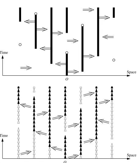
[image:9.612.186.412.86.352.2]Space O
Figure 1: Graphical representation of the contact process and the discretized contact process.
the contact process and the discretized contact process. As explained in more detail in Section 2.2, we prove our main results by proving the results first for the discretized contact process, and then taking the continuum limitǫ↓0.
We denote by(x,s)−→(y,t)the event that(x,s)isconnected to(y,t), i.e., either(x,s) = (y,t)or there is a non-zero path inZd×ǫZ+from(x,s)to(y,t)consisting of occupied bonds. Ther-point
functions, for r≥2,~t= (t1, . . . ,tr−1)∈ǫZr−1
+ and~x = (x1, . . . ,xr−1)∈Zd(r−1), are defined as
τ(r)
~t;ǫ(~x) =P λ
ǫ (o, 0)−→(xi,ti) ∀i=1, . . . ,r−1
. (2.2)
Similarly to (1.6), the discretized contact process has a critical valueλ(ǫ)
c satisfying
ǫ X
t∈ǫZ+ ˆ
τλt;ǫ(0)
(
<∞, ifλ < λ(ǫ)
c ,
=∞, otherwise, limt↑∞P
λ
ǫ(Ct6=∅)
(
=0, ifλ≤λ(ǫ)
c ,
>0, otherwise. (2.3)
The discretization procedure will be essential in order to derive the lace expansion for the r-point functions forr≥3, as it was for the 2-point function in[16].
Note that forǫ=1 the discretized contact process is simply oriented percolation. Our main result for the discretized contact process is the following theorem, similar to Theorem 1.2:
Theorem 2.1(The time-discretized version of Theorem 1.2). (i) Let d > 4, λ = λ(ǫ)
c , r ≥ 2,
~k∈Rd(r−1),~t
∈(0,∞)r−1,δ∈(0, 1∧∆∧d−24)and L ≫1, as in Theorem 1.1(i). There exist A(ǫ)=A(ǫ)(d,L), v(ǫ)=v(ǫ)(d,L), V(ǫ)=V(ǫ)(d,L)such that, for large T ,
ˆ
τ(r)
T~t
~k
p
vσ2T
=A(ǫ) (A(ǫ)
)2V(ǫ) Tr−2
ˆ
M(r−1)
~t (~k) +O(T
where the error term is uniform inǫ∈(0, 1]and in~k in a bounded subset ofRd(r−1). Moreover,
for anyǫ∈(0, 1], λ(ǫ)
c =1+O(L−
d), A(ǫ)=
1+O(L−d), v(ǫ)=
1+O(L−d), V(ǫ)=
2−ǫ+O(L−d). (2.5)
(ii) Let d ≤4, r ≥2,~k ∈Rd(r−1),~t ∈(0,∞)r−1 and letδ,L1,λT,µbe as in Theorem 1.1(ii). For
large T such thatlogT ≥maxiti,
ˆ
τ(r)
T~t
~k
p σ2
TT
= (2−ǫ)Tr−2
ˆ
M~t(r−1)(~k) +O(T−µ∧δ)
, (2.6)
where the error term is uniform inǫ∈(0, 1]and in~k in a bounded subset ofRd(r−1).
Forr=2, the claims in Theorem 2.1 were proved in[16, Propositions 2.1–2.2]. We will only prove the statements forr≥3.
For oriented percolation for whichǫ=1, Theorem 2.1(i) reproves[19, Theorem 1.2]. The unifor-mity inǫ in Theorem 2.1 is crucial in order for the continuum limitǫ↓0 to be performed, and to extend the results to the contact process.
2.2
Overview of the expansion for the higher-point functions
In this section, we give an introduction to the expansion methods of Sections 3–4. For this, it will be convenient to introduce the notation
Λ =Zd
×ǫZ+. (2.7)
We write a typical element of Λ as x rather than (x,t) as was used until now. We fix λ = λ(cǫ)
throughout Section 2.2 for simplicity, though the discussion also applies without change whenλ < λ(ǫ)
c . We begin by discussing the underlying philosophy of the expansion. This philosophy is identical
to the one described in[20, Section 2.2.1].
As explained in more detail in [16], the basic picture underlying the expansion for the 2-point function is that a cluster connectingoand x can be viewed as a string of sausages. In this picture,
the strings joining sausages are the occupied pivotal bonds for the connection fromotox. Pivotal
bonds are the essential bonds for the connection fromotox, in the sense that each occupied path
from o to x must use all the pivotal bonds. Naturally, these pivotal bonds are ordered in time.
Each sausage corresponds to an occupied cluster from the endpoint of a pivotal bond, containing the starting point of the next pivotal bond. Moreover, a sausage consists of two parts: the backbone, which is the set of sites that are along occupied paths from the top of the lower pivotal bond to the bottom of the upper pivotal bond, and the hairs, which are the parts of the cluster that are not connected to the bottom of the upper pivotal bond. The backbone may consist of a single site, but may also consist of sites on at least two bond-disjoint connections. We say that both these cases correspond to double connections. We now extend this picture to the higher-point functions.
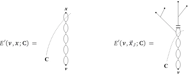
For connections from the origin to multiple points~x = (x1, . . . ,xr−1), the corresponding picture is
a “tree of sausages” as depicted in Figure 2. In the tree of sausages, the strings represent the union overi=1, . . . ,r−1 of the occupied pivotal bonds for the connections o−→xi, and the sausages
are again parts of the cluster between successive pivotal bonds. Some of them may be pivotal for
Í Í Í Í Í Í Í Í Í Í Í Í Í Í Í Í Í Í Í Í Í Í Í Í Í Í Í Í Í Í Í Í Í Í Í Í Í Í Í Í Í Í Í Í Í Í Í Í Í Í Í Í Í Î Î Î Í Í Í Í Í Í Í Í Í Í Í Í Í Í Í Í Í Í Í Í Í Í Í Í Í Í Í Í Î Î Î Î Î Î Î Î Î Î Î Î Î Î Î Î Í Í Í Í Í Í Î Î Î Î Í Í Í Î Î Î Î Î Î Î Î Î Î Î Î Î Î Î Î Î Î Î Î Î Î Î Î Î Î Î Î Î Î Î Î Î Î Î Î Î Î Î Î Î Î Î Í Í Í Í Í Í Í Í Í Î Î Î Î Î Í Í Í Í Í Í Í Î Î Î Î Î Í Í Í Í Í Í Í Î Î Î Í Í Í Í Í Í Í Í Í Í Í Í Í Í Í Í Í Í Í Î Î Î Î Í Í Í Í Í Í Í Í Í Í Í Í Í Í Í Î Î Î Î Î Î Î Í Í Í Í Í Í Í Í Í Í Î Î Î Î Î Î Í Î Î Î Î Î Î Î Î Î Î Î Î Î Î Î Í Í Í Í Í Í Í Í Í Í Í Í Í Í Î Î Î Î Î Î Î Í Í Í Í Í Í Í Í Í Í Í Í Í Í Í Í Í Í Í Í Í Í Í Í Í Í Í Í Í Í Í Í Í Í Í Í Í Í Í Í Í Í Í Í Í ⇐= ⇐= ⇐= =⇒ =⇒ =⇒ =⇒ =⇒ =⇒ ⇐= ⇐= ⇐= ⇐= =⇒ ⇐= ⇐= ⇐= o
x1 x2
o
x1 x2
Figure 2: (a) A configuration for the discretized contact process. Both Î andÍ denote occupied temporal bonds; Î is connected from o, while Í is not. The arrows are occupied spatial bonds,
representing the spread of an infection to neighbours. (b) Schematic depiction of the configuration as a “string of sausages.”
We regard this picture as corresponding to a kind of branching random walk. In this correspondence, the steps of the walk are the pivotal bonds, while the sites of the walk are the backbones between subsequent pivotal bonds. Of course, the pivotal bonds introduce an avoidance interaction on the branching random walk. Indeed, the sausages are not allowed to share sites with the later backbones (since otherwise the pivotal bonds in between would not be pivotal).
When d >4 or when d ≤4 and the range of the contact process is sufficiently large as described in (1.7)–(1.8), the interaction is weak and, in particular, the different parts of the backbone in between different pivotal bonds are small and the steps of the walk are effectively independent. Thus, we can think of the higher-point functions of the critical time-discretized contact process as “small perturbations" of the higher-point functions of critical branching random walk. We will use this picture now to give an informal overview of the expansions we will derive in Sections 3–4.
We start by introducing some notation. Forr≥3, let
J={1, 2, . . . ,r−1}, Jj=J\ {j} (j∈J). (2.8)
ForI ={i1, . . . ,is} ⊂J, we write~xI={xi1, . . . ,xis}and~xI−y ={xi1−y, . . . ,xis−y}and abuse notation by writing
pǫ(x) =pǫ(x)δt,ǫ for x = (x,t). (2.9)
There may be anywhere from 0 tor−1 pivotal bonds, incident to the sausage at the origin, for the event
[image:11.612.91.499.82.285.2]Configurations with zero or more than two pivotal bonds will turn out to constitute an error term. Indeed, when there are zero pivotal bonds, this means thato=⇒xifor eachi, which constitutes an
error term. When there are more than two pivotal bonds, the sausage at the origin has at leastthree
disjoint connections to different xi’s, which also turns out to constitute an error term. Therefore,
we are left with configurations which have one or two branches emerging from the sausage at the origin. When there is one branch, then this branch contains~xJ. When there are two branches, one
branch will contain~xI for some nonemptyI⊆J1and the other branch will contain~xJ\I, where we
require 1∈J\Ito make the identification unique.
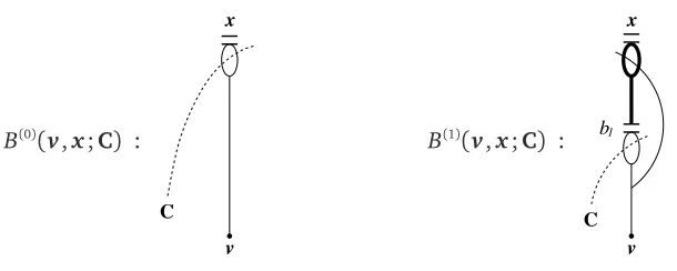
The first expansion deals with the case where there is a single branch from the sausage at the origin. It serves to decouple the interaction between that single branch and the branches of the tree of sausages leading to~xJ. From now on, we write a functionF onΛn≡Zd n×Zn+(or onZd n×Rn+for
the continuous-time model) for a givenn∈Nas
F(~x) =F~t(~x) for ~x = (~x,~t). (2.11)
The expansion writesτ(~xJ)in the form
τ(~xJ) =A(~xJ) + (B⋆τ)(~xJ) =A(~xJ) +
X
v∈Λ
B(v)τ(~xJ−v), (2.12)
where(f⋆g)(x)represents the space-time convolution of two functions f,g:Λ→Rgiven by
(f⋆g)(x) =
X
y∈Λ
f(y)g(x−y). (2.13)
For details, see Section 3, where (2.12) is derived. We have that
B(x) = (π⋆pǫ)(x), (2.14)
where π(x) is the expansion coefficient for the 2-point function as derived in [16, Section 3].
Moreover, forr=2,
A(x) =π(x), (2.15)
so that (2.12) becomes
τ(x) =π(x) + (π⋆pǫ ⋆τ)(x). (2.16)
This is the lace expansion for the 2-point function, which serves as the key ingredient in the analysis of the 2-point function in[16].1
The next step is to writeA(~xJ)as
A(~xJ) =
X
I⊂J1:I6=∅
X
y1
B(y1,~xI)τ(~xJ\I−y1) +a(~xJ; 1), (2.17)
where, to leading order,J\Iconsists of those jfor which the first pivotal bond for the connection to
xj is the same as the one for the connection tox1, while fori∈I, this first pivotal is different. The 1In this paper, we will use a different expansion for the 2-point function than the one used in[16]. However, the
equality (2.17) is the result of thefirst expansion for A(~xJ). In this expansion, we wish to treat the
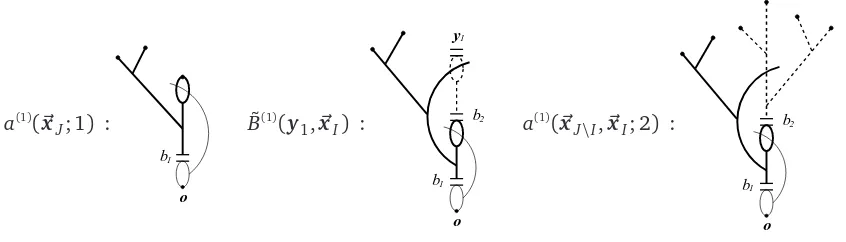
connections from the top of the first pivotal to~xJ\I as being independent from the connections from
oto~xI that do not use the first pivotal bond. In thesecond expansionforA(~xJ), we wish to extract
a factorτ(~xI−y2) for some y2 from the connection fromoto~xI that is still present in B(y1,~xI).
This leads to a result of the form
X
y1
B(y1,~xI)τ(~xJ\I−y1) =
X
y1,y2
C(y1,y2)τ(~xJ\I−y1)τ(~xI−y2) +a(~xJ\I,~xI), (2.18)
wherea(~xJ\I,~xI)is an error term, and, to first approximation,C(y1,y2)represents the sausage ato
together with the pivotal bonds ending aty1andy2, with the two branches removed. In particular,
C(y1,y2)is independent ofI. The leading contribution toC(y1,y2)ispǫ(y1)pǫ(y2)withy16=y2,
corresponding to the case where the sausage at o is the single pointo. For details, see Section 4,
where (2.18) is derived.
We will use a new expansion for the higher-point functions, which is a simplification of the expansion for oriented percolation inZd
×Z+in[20]. The difference resides mainly in the second expansion,
i.e., the expansion ofA(~xJ).
2.3
The main identity and estimates
In this section, we solve the recursion (2.12) by iteration, so that on the right-hand side nor-point function appears. Instead, onlys-point functions withs< r appear, which opens up the possibility for an inductive analysis inr. The argument in this section is virtually identical to the argument in
[19, Section 2.3], and we add it to make the paper self-contained.
We define
ν(x) =
∞
X
n=0
B⋆n(x), (2.19)
whereB⋆n denotes then-fold space-time convolution ofBwith itself, withB⋆0(x) =δo,x. The sum overnin (2.19) terminates after finitely many terms, since by definitionB((x,t))6=0 only ift∈ǫN, so that in particularB((x, 0)) =0. Therefore,B⋆n(x) =0 if n> tx/ǫ, where, for x = (x,t)∈Λ,
tx =t denotes the time coordinate ofx. Then (2.12) can be solved to give
τ(~xJ) = (ν⋆A)(~xJ). (2.20)
The functionν can be identified as follows. We note that (2.20) forr=2 yields that
τ(x) = (ν⋆A)(x). (2.21)
Thus, extracting the n = 0 term from (2.19), using (2.15) to write one factor of B as A⋆pǫ (cf., (2.14)) for the terms withn≥1, it follows from (2.21) that
ν(x) =δo,x+ (ν⋆B)(x) =δo,x+ (ν⋆A⋆pǫ)(x) =δo,x+ (τ⋆pǫ)(x). (2.22)
Substituting (2.22) into (2.20), the solution to (2.12) is then given by
which recovers (2.16) whenr=2, using (2.15). Forr ≥3, we further substitute (2.17)–(2.18) into (2.23). Let
ψ(y1,y2) =
X
v
pǫ(v)C(y1−v,y2−v), (2.24)
ζ(r)
(~xJ) =A(~xJ) + (τ⋆pǫ ⋆a)(~xJ), (2.25)
where
a(~xJ) =a(~xJ; 1) +
X
I⊂J1:I6=∅
a(~xJ\I,~xI). (2.26)
Then, (2.23) becomes
τ(r) (~xJ) =
X
v,y1,y2
τ(2)
(v)ψ(y1−v,y2−v)
X
I⊂J1:I6=∅
τ(r1)(~x
J\I−y1)τ
(r2)(~x
I−y2) +ζ
(r)
(~xJ), (2.27)
wherer1=|J\I|+1 andr2=|I|+1. Since 1≤ |I| ≤r−2, we have thatr1,r2≤r−1, which opens
up the possibility for induction inr.
The first term on the right side of (2.27) is the main term. The leading contribution toψ(y1,y2)is
ψ2ǫ,2ǫ(y1,y2)≡ψ (y1, 2ǫ),(y2, 2ǫ)=X
u
pǫ(u)pǫ(y1−u)pǫ(y2−u) (1−δy1,y2), (2.28)
using the leading contribution toC described below (2.18).
We will analyse (2.27) using the Fourier transform. ForI⊆J, we write
~kI= (ki)i
∈I, kI=
X
i∈I
ki, ~tI= (ti)i∈I, tI=mini∈I ti, (2.29)
and abbreviate them to~k, k, ~t and t, respectively, when I = J. With this notation, the Fourier transform of (2.27) becomes
ˆ
τ(r)
~t (~k) = tX−2ǫ
•
s0=0 ˆ
τ(2)
s0(k)
X
∅6=I⊂J1
tJ\IX−s0 •
s1=2ǫ
tXI−s0 •
s2=2ǫ ˆ
ψs1,s2(kJ\I,kI) ˆτ
(r1)
~tJ\I−s1−s0(
~kJ
\I) ˆτ
(r2)
~tI−s2−s0(
~kI) + ˆζ(r)
~t (~k),
(2.30)
whereP•t≤s≤t′ is an abbreviation for
P
s∈[t,t′]∩ǫZ+. The identity (2.30) is our main identity and will be our point of departure for analysing the r-point functions for r ≥3. Apart fromψandζ(r), the right-hand side of (2.27) involves thes-point functions withs=2,r1,r2. As discussed below (2.27),
we can use an inductive analysis, with ther =2 case given by the result of Theorem 1.1 proved in
[16]. The term involvingψis the main term, whereasζ(r) will turn out to be an error term.
The analysis will be based on the following important proposition, whose proof is deferred to Sec-tions 5–7. In its statement, we denote ∂2
∂k2 by∇
2
k and use the notation
b(ǫ)
s1,s2=
ǫns1,s2
1{s1≤s2} (1+s1)(d−2)/2 ×
(1+s2−s1)−(d−2)/2 (d>2), log(1+s2) (d=2),
(1+s2)(2−d)/2 (d<2),
where
ns1,s2=3−δs1,s2−δs1,2ǫδs2,2ǫ. (2.32) We note that the number of powers ofǫis precisely such that, ford>4,
∞
X•
s1,s2=2ǫ
b(ǫ)
s1,s2=O(ǫ). (2.33)
We also rely on the notation
β=L−d, (2.34)
and, ford≤4, we writeβT =L−
d
T . Then, the main bounds on the lace-expansion coefficients are as follows:
Proposition 2.2(Bounds on the lace-expansion coefficients). The lace-expansion coefficients sat-isfy the following properties:
ψ2ǫ,2ǫ(y1,y2) =X
u
pǫ(u)pǫ(y1−u)pǫ(y2−u) (1−δy1,y2). (2.35)
(i) Let d>4,κ∈(0, 1∧∆∧d−4
2 ),λ=λ
(ǫ)
c and r≥3. There exist Cψ,C
(r)
ζ <∞(independent ofǫ)
and L0=L0(d)such that, for all L≥L0, q∈ {0, 2}, ki ∈[−π,π]d (i=1, . . . ,r−1), si,tj∈ǫZ+
(i=1, 2, j=1, . . . ,r−1), the following bounds hold:
|∇qki ˆ
ψs1,s2(k1,k2)| ≤Cψσq(1+si)q/2(δs1,s2+β)β(b(ǫ)
s1,s2+b
(ǫ)
s2,s1), (2.36)
|ζˆ(r)
~t (~k)| ≤C
(r)
ζ (1+¯t)
r−2−κ, (2.37)
where¯t denote the second-largest element of{t1, . . . ,tr−1}.
(ii) Let d≤4withα≡ bd−4−2d >0,κ∈(0,α)and r≥3. LetβT=β1T−bd andλT=1+O(T−µ)
with µ ∈ (0,α−δ), as in Theorem 1.1(ii). There exist Cψ,C(r)
ζ < ∞(independent of ǫ) and
L0 = L0(d) such that, for L1 ≥ L0 with LT defined as in (1.7), q ∈ {0, 2}, ki ∈ [−π,π]d
(i=1, . . . ,r−1), si,tj≤ǫZ+∩[0, logT](i=1, 2, j=1, . . . ,r−1), the following bounds hold:
|∇qkiψˆs1,s2(k1,k2)| ≤Cψσ
q(1+s
i)q/2(δs1,s2+βT)βT(b
(ǫ)
s1,s2+b
(ǫ)
s2,s1), (2.38)
|ζˆ(r)
~t (~k)| ≤C
(r)
ζ T
r−2−κ. (2.39)
We will prove the identity (2.35) in Section 4.4, the bounds (2.36) and (2.38) in the beginning of Section 6, and the bounds (2.37) and (2.39) in the beginning of Section 7.
It follows from (2.36) and (2.33) that ford>4, the constantV(ǫ) defined by
V(ǫ) = 1
ǫ
∞
X•
s1,s2=2ǫ ˆ
ψs1,s2(0, 0), (2.40)
withλ=λ(ǫ)
c , is finite uniformly inǫ >0. In Proposition 2.4 below, we will prove the existence of
limǫ↓0V(ǫ). The constantV of Theorem 1.2 should then be given by that limit. By (2.28),
O(β)andλ(ǫ)
c =1+O(β)uniformly inǫ, we have
ˆ
ψ2ǫ,2ǫ(0, 0) = (1−ǫ+λ(cǫ)ǫ)
(1−ǫ+λ(ǫ)
c ǫ) 2
−
(1−ǫ)2+ (λ(ǫ)
c ǫ) 2X
x
D(x)2
| {z }
(2−ǫ+O(β)ǫ)λ(cǫ)ǫ
= 2−ǫ+O(β)ǫ.
Combining this with (2.36) yields
V(ǫ)=2
−ǫ+O(β). (2.41)
This establishes the claim onV of Theorem 1.2(i). Ford≤4, on the other hand,β=βT converges to zero asT ↑ ∞, so thatV(ǫ)
is replaced by 2−ǫin Theorem 2.1(ii).
2.4
Induction in
r
In this section, we prove Theorem 2.1 forǫ∈(0, 1]fixed, assuming (2.30) and Proposition 2.2. The argument in this section is an adaptation of the argument in[20, Section 2.3], adapted so as to deal with the uniformity in the time discretization. In particular, in this section, we prove Theorem 2.1 for oriented percolation for whichǫ=1.
Forr≥3, we will use the notation
¯
t =the second-largest element of{t1, . . . ,tr−1}, t=min{t1, . . . ,tr−1}. (2.42)
Proof of Theorem 2.1(i) assuming Proposition 2.2. We prove that for d > 4 there are positive
con-stants L0 = L0(d) andV(ǫ) =V(ǫ)(d,L) such that forλ=λ(cǫ), L ≥ L0 andκ∈(0, 1∧∆∧d−24), we
have
ˆ
τ(r)
~t (
~k
p
v(ǫ)σ2t) =A
(ǫ) (
A(ǫ))2V(ǫ) t)r−2
ˆ
M~(tr/−t1)(~k) +O (¯t+1)−κ (r≥3) (2.43)
uniformly in t ≥¯t and in~k∈R(r−1)d withPir=−11|ki|2 bounded, and uniformly inǫ >0. To prove Theorem 2.1(i), we taket=Tand replace~tbyT~t. Since, without loss of generality, we may assume that maxiti=1 andti≤1, we thus have thatT≥T¯t, so that (2.43) indeed proves Theorem 2.1(i).
We prove (2.43) by induction inr, with the initial case of r=2 given by Theorem 2.1(i):
ˆ
τt1(
k
p
v(ǫ)σ2t) = ˆτt1
kp
t1/t
p
v(ǫ)σ2t 1
=A(ǫ)e− |k|2t
1
2d t +O (t1+1)−κ, (2.44)
using the facts that |k|2 is bounded, t1 ≤ t and κ < d−24. The induction will be advanced using
(2.30). Letr ≥3. By (2.37),ζˆ(r)
~t (~k)is an error term. Thus, we are left to determine the asymptotic
behaviour of the first term on the right-hand side of (2.30).
Fix~kwithPir=−11|ki|2bounded. To abbreviate the notation, we write
~k(t)= ~k p
v(ǫ)σ2t
Given 0≤s0≤t, let t0=s0∧(t−s0). We show that, for every nonempty subsetI⊂J1,
tJX\I−s0 •
s1=2ǫ
tXI−s0 •
s2=2ǫ ˆ
ψs1,s2(k
(t)
J\I,k
(t)
I ) ˆτ
(r1)
~tJ\I−s1−s0(
~k(t)
J\I) ˆτ
(r2)
~tI−s2−s0(
~k(t)
I )−V
(ǫ)ˆ τ(r1)
~tJ\I−s0(
~k(t)
J\I) ˆτ
(r2)
~tI−s0(
~k(t)
I )
≤Cǫtr−3(t
0+1)−κ. (2.46)
Before establishing (2.46), we first show that it implies (2.43). Since|τˆs0(k
(t))
|is uniformly bounded by Theorem 2.1 forr=2, inserting (2.46) into (2.30) and applying (2.37) gives
ˆ
τ(r)
~t (~k
(t)) = V(ǫ)
ǫ
t
X•
s0=0 ˆ
τs0(k
(t)) X
I⊂J1:|I|≥1 ˆ
τ(r1) ~tJ\I−s0(
~k(t)
J\I)ˆτ
(r2)
~tI−s0(
~k(t)
I ) +O(t r−3)ǫ
t
X•
s0=0
(t0+1)−κ+O(tr−2−κ).
(2.47)
Using the fact thatκ <1, the summation in the error term can be seen to be bounded by a multiple oft1−κ≤t1−κ. With the induction hypothesis and the identityr1+r2= r+1, (2.47) then implies that
ˆ
τ(r)
~t (~k
(t)) = A(ǫ) (
A(ǫ))2V(ǫ) tr−2ǫ
t
X•
s0=0 ˆ
Ms(1)
0/t(k)
X
I⊂J1:|I|≥1 ˆ
M(r1−1) ~tJ\I−s0
t
(~kJ\I) ˆM
(r2−1)
~t I−s0 t
(~kI) +O(tr−2−κ),
(2.48)
where the error arising from the error terms in the induction hypothesis again contributes an amount
O(tr−3)ǫX•t
s0=0
(t0+1)−κ≤O(tr−2−κ). The summation on the right-hand side of (2.48), divided by t, is the Riemann sum approximation to an integral. The error in approximating the integral by this Riemann sum isO(ǫt−1). Therefore, using (1.17), we obtain
ˆ
τ(r)
~t (~k
(t) ) =A(ǫ)
(A(ǫ) )2V(ǫ)
tr−2 Z t/t
0
ds0Mˆ(1)
s0(k)
X
I⊂J1:|I|≥1 ˆ
M(r1−1)
~tJ\I−s0 t
(~kJ\I) ˆM(r2−1)
~t I−s0 t
(~kI) +O(tr−2−κ)
=A(ǫ) (A(ǫ))2V(ǫ)tr−2Mˆ(r−1)
~t/t (~k) +O(t
r−2−κ). (2.49)
Sincet≥¯t, it follows that tr−2−κ≤C tr−2(¯t+1)−κ. Thus, it suffices to establish (2.46). To prove (2.46), we write the quantity inside the absolute value signs on the left-hand side as
tJX\I−s0 •
s1=2ǫ
tXI−s0 •
s2=2ǫ ˆ
ψs1,s2(k
(t)
J\I,k
(t)
I ) ˆτ
(r1)
~tJ\I−s1−s0
(~k(Jt\)I) ˆτ(r2) ~tI−s2−s0
(~k(It))−V(ǫ)ˆ τ(r1)
~tJ\I−s0
(~kJ(t\)I) ˆτ(r2) ~tI−s0
(~k(It))
with
T1= ˆτ
(r1)
~tJ\I−s0
(~k(Jt\)I) ˆτ(r2) ~tI−s0
(~k(It))
tJX\I−s0 •
s1=2ǫ
tXI−s0 •
s2=2ǫ ˆ
ψs1,s2(0, 0)−V
(ǫ)
, (2.51)
T2= ˆτ(r1) ~tJ\I−s0(
~k(t)
J\I) ˆτ
(r2) ~tI−s0(
~k(t)
I ) tJX\I−s0
•
s1=2ǫ
tXI−s0 •
s2=2ǫ
ˆ
ψs1,s2(k(Jt\)I,k(It))−ψˆs1,s2(0, 0)
, (2.52)
T3=
tJX\I−s0 •
s1=2ǫ
tXI−s0 •
s2=2ǫ ˆ
ψs1,s2(k(t)
J\I,k
(t)
I )
×
ˆ
τ(r1) ~tJ\I−s1−s0(
~k(t)
J\I) ˆτ
(r2) ~tI−s2−s0(
~k(t)
I )−τˆ
(r1) ~tJ\I−s0(
~k(t)
J\I) ˆτ
(r2) ~tI−s0(
~k(t)
I )
. (2.53)
To complete the proof, it suffices to show that for each nonemptyI⊂J1, the absolute value of each
Ti is bounded above by the right-hand side of (2.46).
In the course of the proof, we will make use of some bounds on sums involving b(ǫ)
s1,s2:
Lemma 2.3(Bounds on sums involving b(ǫ)
s1,s2). (i) Let d > 4. For everyκ∈[0, 1∧
d−4
2 ), there
exists a constant C=C(d,κ)such that the following bounds hold uniformly inǫ∈(0, 1] ∞
X•
s1,s2=2ǫ (s1∨s2≤s)
si(b(sǫ1),s2+b
(ǫ)
s2,s1)≤Cǫ(1+s)
1−κ,
∞
X•
s1,s2=2ǫ (s1∨s2≥s)
b(ǫ)
s1,s2≤Cǫ(1+s)
−κ. (2.54)
(ii) Let d≤4withα≡bd−4−d
2 >0, fixα∈(0,α), recallβT =β1T−bd and letβˆT=β1T−α. There
exists a constant C=C(d,κ)such that the following bound holds uniformly inǫ∈(0, 1]
βT
TXlogT
•
s1,s2=2ǫ (s1∨s2>2ǫ)
(δs1,s2+βT)(b (ǫ)
s1,s2+b
(ǫ)
s2,s1)≤C ˆ
βTǫ. (2.55)
Proof. (i) This is straightforward from (2.31), when we pay special attention to the number of
powers of ǫ present in b(ǫ)
s1,s2 and use the fact that the power of (1+s1) and of (1+s2−s1) is (d−2)/2>1.
(ii) We shall only perform the proof ford<4, as the proof ford =4 is a slight modification of the argument below. Using (2.31), we can perform the sum to obtain
LHS of (2.55)≤O(βT)ǫ
2 X•
2ǫ<s1≤TlogT
(1+s1)(2−d)/2
+O(βT2)ǫ3 X•
2ǫ≤s1<s2≤TlogT
(1+s1)(2−d)/2(1+s2−s1)(2−d)/2
≤O(βT)ǫ 1+TlogT
(4−d)/2
1+βT 1+TlogT
(4−d)/2
≤O( ˆβT)ǫ(1+ ˆβT), (2.56)
We now resume proving (2.46). By the induction hypothesis and the fact that ¯tI
i ≤t, it follows that
|τˆ(~tri) Ii(
~kI
i)| ≤O(t
ri−2)uniformly in~t
Ii and~kIi. Therefore, it follows from (2.36) and the definition of
V(ǫ)in (2.40) that
|T1| ≤
X•
s1≥tJ\I−s0
or
s2≥tI−s0
O(tr−3)b(ǫ)
s1,s2≤O(ǫt
r−3(t
0+1)−
(d−4)/2), (2.57)
where the final bound follows from the second bound in (2.54).
Similarly, by (2.36) withq=2, now using the first bound in (2.54),
|T2| ≤
tJX\I−s0 •
s1=2ǫ
tXI−s0 •
s2=2ǫ (s1|k(t)
J\I|
2+s 2|k
(t)
I |
2)O(tr−3)b(ǫ)
s1,s2≤O(ǫt
r−3(t
0+1)−
κ), (2.58)
using that tr−4(t0+1)1−κ≤tr−3(t0+1)−κsince t≥t0. It remains to prove that
|T3| ≤O(ǫtr−3(t0+1)−κ). (2.59)
To begin the proof of (2.59), we note that the domain of summation overs1,s2in (2.53) is contained in∪2
j=0Sj(~t), where
S0(~t) = [0, 12(tJ\I−s0)]×[0, 12(tI−s0)],
S1(~t) = [12(tJ\I−s0), tJ\I−s0]×[0,tI−s0],
S2(~t) = [0,tJ\I−s0]×[12(tI−s0), tI−s0].
Therefore,|T3|is bounded by
2
X
j=0
X•
~s∈Sj(~t)
ψˆ
s1,s2(k
(t)
J\I,k
(t)
I )
τˆ(r1)
~tJ\I−s1−s0
(~k(Jt\)I)ˆτ(r2) ~tI−s2−s0
(~k(It))−τˆ(r1) ~tJ\I−s0
(~k(Jt\)I)ˆτ(r2) ~tI−s0
(~k(It))
. (2.60)
The terms with j = 1, 2 in (2.60) can be estimated as in the bound (2.57) on T1, after using the triangle inequality and bounding theri-point functions byO(tri−2).
For the j=0 term of (2.60), we write
ˆ
τ(r1) ~tJ\I−<