El e c t ro n ic
Jo ur n
a l o
f P
r o b
a b i l i t y Vol. 11 (2006), Paper no. 30, pages 768–801.
Journal URL
http://www.math.washington.edu/~ejpecp/
Convergence results and sharp estimates for the
voter model interfaces
S. Belhaouari ´
Ecole Polyt´echnique F´ederale de Lausanne (EPFL)
1015, Lausanne, Switzerland e-mail: [email protected]
T. Mountford ´
Ecole Polyt´echnique F´ederale de Lausanne (EPFL)
1015, Lausanne, Switzerland e-mail: [email protected]
Rongfeng Sun
EURANDOM, P.O. Box 513 5600 MB Eindhoven, The Netherlands
e-mail: [email protected]
G. Valle ´
Ecole Polyt´echnique F´ederale de Lausanne (EPFL)
1015, Lausanne, Switzerland e-mail: [email protected]
Abstract
We study the evolution of the interface for the one-dimensional voter model. We show that if the random walk kernel associated with the voter model has finiteγth moment for some γ >3, then the evolution of the interface boundaries converge weakly to a Brownian motion under diffusive scaling. This extends recent work of Newman, Ravishankar and Sun. Our result is optimal in the sense that finite γth moment is necessary for this convergence for allγ ∈(0,3). We also obtain relatively sharp estimates for the tail distribution of the size of the equilibrium interface, extending earlier results of Cox and Durrett, and Belhaouari, Mountford and Valle
Key words: voter model interface, coalescing random walks, Brownian web, invariance principle
1
Introduction
In this article we consider the one-dimensional voter model specified by a random walk transition kernelq(·,·), which is an Interacting Particle System with configuration space Ω ={0,1}Z
and is formally described by the generator G acting on local functions F : Ω→ R (i.e., F depends
on only a finite number of coordinates ofZ),
(GF)(η) =X
x∈Z
X
y∈Z
q(x, y)1{η(x)6=η(y)}[F(ηx)−F(η)], η∈Ω
where
ηx(z) =
η(z), ifz6=x
1−η(z), ifz=x .
By a result of Liggett (see [7]),G is the generator of a Feller process (ηt)t≥0 on Ω. In this paper
we will also impose the following conditions on the transition kernel q(·,·):
(i) q(·,·) is translation invariant, i.e., there exists a probability kernel p(·) on Z such that q(x, y) =p(y−x) for allx, y ∈Z.
(ii) The probability kernelp(·) is irreducible, i.e., {x:p(x)>0} generates Z.
(iii) There exists γ ≥1 such thatP
x∈Z|x|γp(x)<+∞.
Later on we will fix the values ofγ according to the results we aim to prove. We also denote by
µthe first moment of p
µ:=X
x∈Z xp(x),
which exists by (iii).
Letη1,0 be the Heavyside configuration on Ω, i.e., the configuration:
η1,0(z) =
1, ifz≤0 0, ifz≥1,
and consider the voter model (ηt)t≥0 starting atη1,0. For each timet >0, let
rt= sup{x:ηt(x) = 1} and lt= inf{x:ηt(x) = 0},
which are respectively the positions of the rightmost 1 and the leftmost 0. We call the voter model configuration between the coordinateslt andrtthe voter model interface, and rt−lt+ 1
is the interface size. Note that condition (iii) on the probability kernel p(·) implies that the interfaces are almost surely finite for allt≥0 and thus well defined. To see this, we first observe that the rate at which the interface size increases is bounded above by
X
x<0<y
{p(y−x) +p(x−y)}=X
z∈Z
|z|p(z)<∞. (1.1)
When γ ≥ 2, Belhaouari, Mountford and Valle [1] proved that the interface is tight, i.e., the random variables (rt−lt)t≥0 are tight. This extends earlier work of Cox and Durrett [4], which
showed the tightness result when γ ≥3. Belhaouari, Mountford and Valle also showed that, if
P
x∈Z|x|γp(x) = ∞ for some γ ∈ (0,2), then the tightness result fails. Thus second moment
is, in some sense, optimal. Note that the tightness of the interface is a feature of the one-dimensional model. For voter models in dimension two or more, the so-called hybrid zone grows as√tas was shown in [4].
In this paper we examine two questions for the voter model interface: the evolution of the interface boundaries, and the tail behavior of the equilibrium distribution of the interface which is known to exist whenever the interface is tight. Third moment will turn out to be critical in these cases.
From now on we will assumep(·) is symmetric, and in particularµ= 0, which is by no means a restriction on our results since the general case is obtained by subtracting the drift and working with the symmetric part ofp(·):
ps(x) = p(x) +p(−x)
2 .
The first question arises from the observation of Cox and Durrett [4] that, if (rt−ℓt)t≥0 is tight,
then the finite-dimensional distributions of
r
tN2
N
t≥0 and
ltN2
N
t≥0
converge to those of a Brownian motion with speed
σ := X
z∈Z z2p(z)
!1/2
. (1.2)
As usual, let D([0,+∞),R) be the space of right continuous functions with left limits from [0,+∞) to R, endowed with the Skorohod topology. The question we address is, as N → ∞,
whether or not the distributions onD([0,+∞),R) of
r
tN2
N
t≥0 and
ltN2
N
t≥0
converge weakly to a one-dimensionalσ-speed Brownian Motion, i.e, (σBt)t≥0, where (Bt)t≥0 is
a standard one-dimensional Brownian Motion. We show:
Theorem 1.1. For the one-dimensional voter model defined as above
(i) If γ >3, then the path distributions on D([0,+∞),R) of
r
tN2
N
t≥0 and
ltN2
N
t≥0
(ii) For (rtN2
N )t≥0
resp. (ltN2
N )t≥0
to converge to a Brownian motion, it is necessary that
X
x∈Z
|x|3
logβ(|x| ∨2)p(x)<∞ for all β >1.
In particular, if for some 1 ≤ γ < γ <˜ 3 we have P
x|x|γ˜p(x) = ∞, then {( rtN2
N )t≥0}
resp. (ltN2
N )t≥0
is not a tight family in D([0,+∞),R), and hence cannot converge in
distribution to a Brownian motion.
Remark 1. Theorem 1.1(i) extends a recent result of Newman, Ravishankar and Sun [9], in which they obtained the same result for γ ≥ 5 as a corollary of the convergence of systems of coalescing random walks to the so-called Brownian web under a finite fifth moment assumption. The difficulty in establishing Theorem1.1(i) and the convergence of coalescing random walks to the Brownian web lie both in tightness. In fact the tightness conditions for the two convergences are essentially equivalent. Consequently, we can improve the convergence of coalescing random walks to the Brownian web from a finite fifth moment assumption to a finite γth assumption for anyγ >3. We formulate this as a theorem.
Theorem 1.2. LetX1 denote the random set of continuous time rate 1 coalescing random walk
paths with one walker starting from every point on the space-time latticeZ×R, where the random walk increments all have distributionp(·). LetXδ denote X1 diffusively rescaled, i.e., scale space
by δ/σ and time by δ2. If γ > 3, then in the topology of the Brownian web [9], Xδ converges
weakly to the standard Brownian web W¯ as δ →0. A necessary condition for this convergence is again P
x∈Z
|x|3
logβ(|x|∨2)p(x)<∞ for all β >1.
It should be noted that the failure of convergence to a Brownian motion does not preclude the existence of Ni ↑ ∞ such that
rN2 it
Ni
t≥0 converges to a Brownian motion. Loss of tightness is
due to “unreasonable” large jumps. Theorem 1.3 below shows that, when 2< γ < 3, tightness can be restored by suppressing rare large jumps near the voter model interface, and again we have convergence of the boundary of the voter model interface to a Brownian motion.
Before stating Theorem 1.3, we fix some notation and recall a usual construction of the voter model. We start with the construction of the voter model through the Harris system. Let
{Nx,y}
x,y∈Z be independent Poisson point processes with intensity p(y−x) for each x, y ∈ Z.
From an initial configurationη0 in Ω, we set at time t∈ Nx,y:
ηt(z) =
ηt−(z), ifz6=x
ηt−(y), ifz=x .
From the same Poisson point processes, we construct the system of coalescing random walks as follows. We can think of the Poisson points inNx,y as marks at site x occurring at the Poisson
times. For each space-time point (x, t) we start a random walkXx,t evolving backward in time
such that whenever the walk hits a mark inNu,v(i.e., fors∈(0, t), (t−s)∈ Nu,v andu=Xx,t s ),
space-time point where they first met. We define by ζs the Markov process which describes the
positions of the coalescing particles at times. Ifζs starts at timetwith one particle from every
site of Afor someA⊂Z, then we use the notation
ζst(A) :={Xsx,t:x∈A},
where the superscript is the time in the voter model when the walks first started, and the subscript is the time for the coalescing random walks. It is well known that ζt is the dual
process ofηt(see Liggett’s book [7]), and we obtain directly from the Harris construction that
{ηt(·)≡1 onA}={η0(·)≡1 onζtt(A)}
for all A⊂Z.
Theorem 1.3. Take 2 < γ <3 and fix 0< θ < γ−γ2. For N ≥1, let (ηtN)t≥0 be described as
the voter model according to the same Harris system and also starting from η1,0 except that a
flip from 0 to 1 at a site x at time t is suppressed if it results from the “influence” of a site y
with |x−y| ≥N1−θ and [x∧y, x∨y]∩[rNt−−N, rNt−]6=φ, where rNt is the rightmost 1 for the processη·N. Then
(i)
rN tN2
N
t≥0
converge in distribution to a σ-speed Brownian Motion withσ defined in (1.2).
(ii) As N → ∞, the integral
1
N2
Z T N2
0
IrN s 6=rsds
tends to0 in probability for all T >0.
Remark 2. There is no novelty in claiming that for (rtN2
N )t≥0, there is a sequence of processes
(γN
t )t≥0which converges in distribution to a Brownian motion, such that with probability tending
to 1 asN tends to infinity, γtN is close to rtN2
N most of the time. The value of the previous result
is in the fact that there is a very natural candidate for such a process. Thus the main interest of Theorem 1.3 lies in the lower bound θ > 0. By truncating jumps of size at least N1−θ for
some fixed θ > 0, the tightness of the interface boundary evolution {(r
N tN2
N )t≥0}N∈N is restored.
The upper bound θ < γ−γ2 simply says that with higher moments, we can truncate more jumps without affecting the limiting distribution.
Let {Θx : Ω → Ω, x ∈ Z} be the group of translations on Ω, i.e., (η◦Θx)(y) = η(y+x) for
everyx ∈Z and η ∈Ω. The second question we address concerns the equilibrium distribution
of thevoter model interface (ηt◦Θℓt)t≥0, when such an equilibrium exists. Cox and Durrett [4]
observed that (ηt◦Θℓt|N)t≥0, the configuration ofηt◦Θℓt restricted to the positive coordinates,
evolves as an irreducible Markov chain with countable state space
˜ Ω =
ξ ∈ {0,1}N
:X
x≥1
ξ(x)<∞
Therefore a unique equilibrium distribution π exists for (ηt◦Θℓt|N)t≥0 if and only if it is a
positive recurrent Markov chain. Cox and Durret proved that, when the probability kernelp(·) has finite third moment, (ηt◦Θℓt|N)t≥0 is indeed positive recurrent and a unique equilibrium π exists. Belhaouari, Mountford and Valle [1] recently extended this result to kernels p(·) with finite second moment, which was shown to be optimal.
Cox and Durrett also noted that if the equilibrium distributionπexists, then excluding the trivial nearest neighbor case, the equilibrium has Eπ[Γ] = ∞ where Γ = Γ(ξ) = sup{x :ξ(x) = 1} for
ξ ∈Ω is the interface size. In fact, as we will see, under finite second moment assumpt ion on˜ the probability kernelp(·), there exists a constantC =Cp ∈(0,∞) such that
π{ξ : Γ(ξ)≥M} ≥ Cp
M for all M ∈N,
extending Theorem 6 of Cox and Durrett [4]. Furthermore, we show that M−1 is the correct order forπ{η : Γ(η)≥M}asM tends to infinity ifp(·) possesses a moment strictly higher than 3, but not so ifp(·) fails to have a moment strictly less than 3.
Theorem 1.4. For the non-nearest neighbor one-dimensional voter model defined as above
(i) If γ ≥2, then there exists C1>0 such that for all M ∈N
π{ξ: Γ(ξ)≥M} ≥ C1
M . (1.3)
(ii) If γ >3, then there exists C2>0 such that for all M ∈N
π{ξ: Γ(ξ)≥M} ≤ C2
M . (1.4)
(iii) Let α= sup{γ :P
x∈Z|x|γp(x)<∞}. If α∈(2,3), then
lim sup
n→∞
logπ{ξ: Γ(ξ)≥n}
logn ≥2−α. (1.5)
Furthermore, there exist choices ofp(·) =pα(·) with α∈(2,3) and
π{ξ : Γ(ξ)≥n} ≥ C
nα−2 (1.6)
for some constant C >0.
2
Proof of Theorem
1.1
and
1.2
By standard results for convergence of distributions on the path space D([0,+∞),R) (see for
instance Billingsley’s book [3], Chapter 3), we have that the convergence to theσ-speed Brownian Motion in Theorem 1.1is a consequence of the following results:
Lemma 2.1. If γ ≥2, then for every n ∈ N and 0 < t1 < t2 < ... < tn in [0,∞) the
finite-converges weakly to a centeredn-dimensional Gaussian vector of covariance matrix equal to the identity. Moreover the same holds if we replacert by lt.
Proposition 2.2. If γ >3, then for everyǫ >0 andT >0
In particular if the finite-dimensional distributions of rtN2
N
t≥0 are tight, we have that the path
distribution is also tight and every limit point is concentrated on continuous paths. The same holds if we replacert by lt.
By Lemma2.1and Proposition 2.2we have Theorem 1.1.
Lemma2.1is a simple consequence of the Markov property, the observations of Cox and Durrett [4] and Theorem 2 of Belhaouari-Mountford-Valle [1] where it was shown that for γ ≥ 2 the distribution of rtN2
σN converges to a standard normal random variable (see also Theorem 5 in Cox
and Durrett [4] where the caseγ ≥3 was initially considered).
We are only going to carry out the proof of (2.1) forrtsince the result of the proposition follows
forlt by interchanging the roles of 0’s and 1’s in the voter model.
Note that by the right continuity ofrt, the event in (2.1) is included in
By the Markov property, the attractivity of the voter model and the tightness of the voter model interface, (2.1) is therefore a consequence of the following result: for allǫ >0
Let us first remark that in order to show (2.2) it is sufficient to show that
lim sup
δ→0
δ−1 lim sup
N→+∞
P
"
sup
0≤t≤N2δ
rt≥ǫN
#
= 0. (2.3)
Indeed, from the last equation we obtain
lim sup
δ→0
δ−1 lim sup
N→+∞
P
inf
0≤t≤N2δrt≤ −ǫN
= 0. (2.4)
To see this note thatrt≥lt−1, thus (2.4) is a consequence of
lim sup
δ→0
δ−1 lim sup
N→+∞
P
inf
0≤t≤N2δlt≤ −ǫN
= 0, (2.5)
which is equivalent to (2.3) by interchanging the 0’s and 1’s in the voter model.
The proof of (2.3) to be presented is based on a chain argument for the dual coalescing random walks process. We first observe that by duality, (2.3) is equivalent to showing that for allǫ >0,
lim
δ→0 δ
−1 lim sup
N→+∞
P
ζtt([ǫN,+∞))∩(−∞,0]6=φ for somet∈[0, δN2]
= 0.
Now, if we takeR:=R(δ, N) =√δN and M =ǫ/√δ, we may rewrite the last expression as
lim
M→+∞M
2 lim sup
R→+∞
P
ζtt([M R,+∞))∩(−∞,0]6=φ for somet∈[0, R2]
= 0,
which means that we have to estimate the probability that no dual coalescing random walk starting at a site in [M R,+∞) at a time in the interval [0, R2] arrives at timet= 0 at a site to the left of the origin. It is easy to check that the condition above, and hence Proposition 2.2is a consequence of the following:
Proposition 2.3. If γ > 3, then for R > 0 sufficiently large and 2b ≤ M < 2b+1, for some b∈N the probability
P
ζtt([M R,+∞))∩(−∞,0]6=φ for some t∈[0, R2]
is bounded above by a constant times
X
k≥b
1
22kRγ−23
+e−c2k+ 2kR4e−c2k(1−β)R
(1−β) 2
+ 2ke−c22k
(2.6)
for some c >0 and0< β <1.
Proof:
✁✂✄☎✆✁✝✞✟✠✡ ✂✄☎✆✁✝✞
✡ ✠✡
☎☞ ✌✝✞
✡ ✍✎
✡✏✑ ✍
✆✁✒✓
✂✁✝✞ ✡
✠✡
✁✒✔ ✡
✓ ✁✄
✌✝ ✍✎
✡✏✑ ✍
✆✁✒✓ ✕
✁✒✓
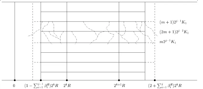
Figure 1: Illustration of thej-th step of the chain argument.
some backward random walk starting from [2kR,2k+1R]×[0, R2] (k≥b) hits the negative axis at time 0. Therefore it suffices to consider such events.
The first step is to discard the event that at least one of the backward coalescing random walks
Xx,s starting in I
k,R = [2kR,2k+1R]×[0, R2] has escaped from a small neighborhood around
Ik,R before reaching time level K1⌊Ks1⌋, where ⌊x⌋ = max{m ∈Z :m ≤x}. The constant K1
will be chosen later. We call this small neighborhood aroundIk,R thefirst-step interval, and the
times {nK1}0≤n≤⌊R2 K1⌋
the first-step times. So after this first step we just have to consider the system of coalescing random walks starting on each site of the first-step interval at each of the first-step times.
In the second step of our argument, we let these particles evolve backward in time until they reach the second-step times: {n(2K1)}0≤n≤⌊R2
2K1⌋
. I.e., if a walk starts at time lK1, we let it
evolve until time (l−1)K1 ifl is odd, and until time (l−2)K1 ifl is even. We then discard the event that either some of these particles have escaped from a small neighborhood around the first-step interval, which we call thesecond-step interval, or the density of the particles alive at each of the second-step times in the second-step interval has not been reduced by a fixed factor 0< p <1.
We now continue by induction. In thejth-step, (see Figure1) we have particles starting from the (j−1)th-step interval with density at mostpj−2 at each of the (j−1)th-step times. We let these
particles evolve backward in time until the next jth-step times: {n(2j−1K1)}0≤n≤⌊ R2 2j−1K1⌋
. We
then discard the event that either some of these particles have escaped from a small neighborhood around the (j−1)th-step interval, which we call the jth-step interval, or the density of the particles alive at each of thejth-step times in the jth-step interval has not been reduced below
pj−1.
We repeat this procedure until theJth-step withJ of order logR, when the onlyJth-step time
left in [0, R2] is 0. The rate p will be chosen such that at the Jth-step, the number of particles alive at time 0 is of the order of a constant which is uniformly bounded in R but which still depends on k. TheJth-step intervalwill be chosen to be contained in [0,3·2kR].
We now give the details. In our approach the factor p is taken to be 2−1/2. The constant
the reduction in the number of particles. Note thatK1is independent ofkandR. Thejth-step interval is obtained from the (j−1)th-step intervals by adding intervals of lengthβjR2kR, where
βRJR−j = 1 2(j+ 1)2,
and
JR= 1 +
1 log 2log
R2 K1
is taken to be the last step in the chain argument. Here⌈x⌉= min{m ∈Z:m ≥x}. We have
chosenJR because it is the step when 2JR−1K1 first exceedsR2 and the only JRth-step time in
[0, R2] is 0. With our choice of βR
j , we have that the JRth-step interval lies within [0,3(2kR)],
and except for the events we discard, no random walk reaches level 0 before time 0.
Let us fix γ = 3 +ǫ in Theorem 1.1. The first step in the chain argument described above is carried out by noting that the event we reject is a subset of the event
n
For somek≥band (x, s)∈[2kR,2k+1R]×[0, R2],
|Xux,s−x| ≥β1R2kR for some 0≤u≤s−K1
s K1
o
.
SinceβR
1 = 1/(2JR2)≥C/(logR)2, Lemma5.5implies that the probability of the above event is
bounded by
X
k≥b
CK1(logR)2(3+ǫ)
22k+3ǫRǫ (2.7)
for R sufficiently large. Therefore, for each k ≥ b, instead of considering all the coalescing random walks starting from [2kR,2k+1R]×[0, R2], we just have to consider coalescing random walks starting from [(1−βR
1)2kR,(2 +β1R)2kR]× {nK1}where{nK1}0≤n≤⌊R2 K1⌋
are the first-step
times. By this observation, we only need to bound the probability of the event
Ak,R =nXx,nK1
u ≤0 for somen= 1, ...,
R2 K1
, u∈[0, nK1]
and x∈h 1−βR1
2kR, 2 +β1R
2kRio.
We start by defining events which will allow us to writeAk,Rin a convenient way. Forn1 :=n∈N
and for each 1≤j ≤JR−1, define recursively
nj+1=
( jn
j−1 2j
k
2j, if jnj−1 2j
k
2j ≥0 0, otherwise .
For a random walk starting at time nK1 in the dual voter model, njK1 is its time coordinate
after the jth step of our chain argument. Then define
W1k,R = n|Xx,nK1
u −x| ≥β2R2kR for somen= 1, ...,
R2 K1
,
u∈[0,(n−n2)K1] and x∈h 1−β1R
2kR, 2 +β1R
and for each 2≤j ≤JR−1
Note that Wjk,R is the event that in the (j+ 1)th step of the chain argument, some random walk starting from ajth-step time makes an excursion of sizeβjR+12kR before it reaches the next (j+ 1)th-step time. Then we have
j the random walks remain confined in the interval
"
coalescing random walks starting at (x, s)∈
1−β1R
Ujk,R is the event that after the (j+ 1)th-step of the chain argument, the density of particles in the (j+ 1)th-step interval at some of the (j+ 1)th-step times {n2jK
1}0≤n≤⌊ R2 2j K1⌋
is greater
than 2−j2. The chain argument simply comes from the following decomposition:
JR−1
We are going to estimate the probability of the events in (2.8) and (2.9).
t1 and t2 are inside the jth-step interval with density at most 2− j−1
2 , and in the (j+ 1)th-step
these walks stay within the (j+ 1)th-step interval until the (j+ 1)th-step time t0 = m2jK1,
when the density of remaining walks in the (j+ 1)th-step interval exceeds 2−j2. We estimate the
probability of this last event by applying three times Proposition5.4 withp= 2−12 andL equal
to the size of the (j+ 1)th-step interval, which we denote by Lk,Rj+1.
We may suppose that at most 2−j−21Lk.R
j+1 random walks are leaving from timest1 andt2. We let
both sets of walks evolve for a dual time interval of length 7−1·2j−1K1= 2j−1K0. By applying Proposition 5.4 with γ = 2−j−21, the density of particles starting at times t1 or t2 is reduced
by a factor of 2−12 with large probability. Now we let the particles evolve further for a t ime
interval of length 2jK
0. Apply Proposition5.4withγ = 2− j
2, the density of remaining particles
is reduced by another factor of 2−12 with large probability. By a last application of Proposition 5.4for another time interval of length 2j+1K0 withγ = 2−
j+1
2 we obtain that the total density of
random walks originating from the twojth-step times t1 (resp. t2) remaining at time t0 (resp. t1) has been reduced by a factor 2−
3
2. Finally we let the random walks remaining at time t1
evolve un till the (j+ 1)th-step time t0, at which time the density of random walks has been
reduced by a factor 2·2−32 = 2− 1
2 with large probability. By a decomposition similar to (2.8) and
(2.9) and using the Markov property, we can assume that before each application of Proposition
5.4, the random walks are all confined within the (j+1)th-step interval. All the events described above have probability at least 1−Ce−c22j/k R2. Since there are (⌊ R2
2jK1⌋+ 1) (j+ 1)th-step times,
the probability of the event in (2.9) is bounded by
C
It is simple to verify that this last expression is bounded above by
C
are contained in thejth-step interval with density at most 2−j−21, and some of these walks move
bounds the number of walks we are considering. By Lemma 5.1 the probability in (2.10) is dominated by a constant times
exp
Then multiplying by (2.11) and summing over 1 ≤ j ≤ JR, we obtain by straightforward
computations that ifRis sufficiently large, then there exist constantsc >0 andc′ >1 such that
the probability of the event in (2.8) is bounded above by a constant times
2kR4e−c2(1−β)kR
Adjusting the terms in the last expression we complete the proof of the proposition.
Proof of (ii) in Theorem 1.1:
For the rescaled voter model interface boundaries ltN2
N and
rtN2
N to converge to aσ-speed
Brow-nian motion, it is necessary that the boundaries cannot wander too far within a small period of time, i.e., we must have
lim
In terms of the dual system of coalescing random walks, this is equivalent to
lim
t→0lim supN→∞ P
ζss([ǫN,+∞))∩(−∞,0]6=φ for somes∈[0, tN2] = 0 (2.14)
and the same statement for its mirror event. If some random walk jump originating from the region [ǫσN,∞)×[0, tN2] jumps across level 0 in one step (which we denote as the event DN(ǫ, t)), then with probability at leastα for someα >0 depending only on the random walk
kernelp(·), that random walk will land on the negative axis at time 0 (in the dual voter model). Thus (2.14) implies that
lim
t→0lim supN→∞ P[DN(ǫ, t)] = 0 (2.15)
Let H(y) = y3log−β(y∨2) for some β > 0. Let H(1)(k) = H(k)−H(k−1) and H(2)(k) =
H(1)(k)−H(1)(k−1) =H(k)+H(k−2)−2H(k−1), which are the discrete gradient and laplacian of H. Then fork≥k0 for somek0 ∈Z+, 0< H(2)(k)<8klog−βk. Denote G(k) =P∞i=kF(i).
Then (2.16) is the same as G(k) ≤ Cǫ
k2 for all k ∈Z+. Recall that ps(k) =
p(k)+p(−k)
2 , we have
by summation by parts
X
k∈Z
H(|k|)p(k) =
∞ X
k=1
2H(k)ps(k)
=
k0−1
X
k=1
2H(k)ps(k) +H(k0)F(k0) +
∞ X
k=k0+1
H(1)(k)F(k)
=
k0−1
X
k=1
2H(k)ps(k) +H(k0)F(k0)
+H(1)(k0+ 1)G(k0+ 1) +
∞ X
k=k0+2
H(2)(k)G(k)
≤
k0−1
X
k=1
2H(k)ps(k) +H(k0)F(k0)
+H(1)(k0+ 1)G(k0+ 1) +
∞ X
k=k0+2
8k
logβk· Cǫ
k2 < ∞
forβ >1. This concludes the proof.
We end this section with
Proof of Theorem 1.2: In [5, 6], the standard Brownian web ¯W is defined as a random variable taking values in the space of compact sets of paths (see [5, 6] for more details), which is essentially a system of one-dimensional coalescing Brownian motions with one Brownian path starting from every space-time point. In [9], it was shown that under diffusive scaling, the random set of coalescing random walk paths with one walker starting from every point on the space-time lattice Z×Z converges to ¯W in the topology of the Brownian web (the details for
the continuous time walks case is given in [11]), provided that the random walk jump kernelp(·) has finite fifth moment. To improve their result from finite fifth moment to finite γ-th moment for any γ > 3, we only need to verify the tightness criterion (T1) formulated in [9], the other
convergence criteria require either only finite second moment or tightness. Recall the tightness criteria (T1) in [9],
(T1) lim
t↓0
1
t lim supδ↓0
sup
(x0,t0)∈ΛL,T
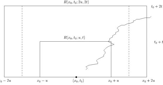
µδ(At,u(x0, t0)) = 0, ∀u >0,
where ΛL,T = [−L, L]×[−T, T], µδ is the distribution of Xδ, R(x0, t0;u, t) is the rectangle
✁✂✄ ✁☎✄ ✁☎✆✄ ✁✂✆✄
✝✞ ✁✟✠✁✡✄✟✠☛ ✁✟✠✁✡✆✄✟✆✠☛
✠✁☎✆✠
✠✁☎✠
✞ ✁✟✠✁☛
Figure 2: Illustration of the eventAt,u(x0, t0).
of coalescing walk paths contains a path touching both R(x0, t0;u, t) and (at a later time) the
left or right boundary of the bigger rectangle R(x0, t0; 2u,2t). In [9], in order to guarantee the
continuity of paths, the random walk paths are taken to be the interpolation between consecutive space-time points where jumps take place. Thus the contribution to the event At,u(x0, t0) is
either due to interpolated line segments intersecting the inner rectangle R(x0, t0;u, t) and then
not landing inside the intermediate rectangle R(x0, t0; 3u/2,2t), which can be shown to have 0
probability in the limitδ→0 if p(·) has finite third moment; or it is due to some random walk originating from inside R(x0, t0; 3u/2,2t) and then reaches either level −2u or 2u before time
2t. In terms of the unscaled random walk paths, and note the symmetry between left and right boundaries, condition (T1) reduces to
lim
t↓0
1
tlim supδ→0 P
ζs1
s2([
uσ
2δ,
7uσ
2δ ])∩(−∞,0]6=φfor some 0≤s2< s1 ≤ t δ2
= 0,
which by the reflection principle for random walks is further implied by
lim
t↓0
1
tlim supδ→0 P
ζss([uσ 2δ,
7uσ
2δ ])∩(−∞,0]6=φfor some 0≤s≤ t δ2
= 0,
which is a direct consequence of Proposition2.3. This establishes the first part of Theorem 1.2. It is easily seen that the tightness of {Xδ} imposes certain equicontinuity conditions on the
random walk paths, and the condition in (2.15) and its mirror statement are also necessary for the tightness of{Xδ}, and hence the convergence ofXδ (with δ= N1) to the standard Brownian
web ¯W. Therefore, we must also haveP
x∈Z
|x|3
logβ(|x|∨2)p(x)<∞for all β >1.
3
Proof of Theorem
1.3
In this section we assume that 2< γ <3 and we fix 0< θ < γ−γ2.
We recall the definition of (ηN
t )t≥0 on Ω. The evolution of this process is described by the
same Harris system on which we constructed (ηt)t≥0, i.e., the family of Poisson point processes
[rNt−−N, rNt−]6=φ, then a flip from 0 to 1 atxory, if it should occur, is suppressed. We also let (ηtN)t≥0 start from the Heavyside configuration η1,0. We also recall that we denote by rNt the
position of its rightmost ”1”.
Since (ηt)t≥0 and (ηtN)t≥0 are generated by the same Harris system and they start with the same
configuration, it is natural to believe thatrN
t =rt for ”most” 0≤t≤N2 with high probability.
To see this we use the additive structure of the voter model to show (ii) in Theorem 1.3.
For a fixed realization of the process (ηNt )t≥0, we denote by t1 < ... < tk the times of the
suppressed jumps in the time interval [0, T N2] and by x1, ..., xk the target sites, i.e., the sites
where the suppressed flips should have occurred. Now let (ηti,xi
t )t≥0 be voter models constructed
on the same Harris system starting at time ti with a single 1 at site xi. As usual we denote by
rti,xi
t ,t≥ti, the position of the rightmost ”1”. It is straightforward to verify that
0≤rt−rNt = max1≤i≤k
ti≤t
(rti,xi
t −rNt )∨0.
The random set of times{ti} is a Poisson point process on [0, N2] with rate at most
X
[x,y]∩[−N,0]6=φ y−x≥N1−θ
{p(y−x) +p(x−y)} ≤ X |x|≥N1−θ
|x|p(x) + (N + 1) X
|x|≥N1−θ p(x),
which is further bounded by
2P
x∈Z|x|αp(x) N(1−θ)α−1
for every α >1. Therefore if we take α =γ, then by the choice of θ and the assumption that theγ-moment of the transition probability is finite, we have that the rate decreases asN−(1+ǫ)
forǫ= (1−θ)γ−2>0.
Lemma 3.1. Let {(ti, xi)}i∈N with t1< t2<· · · denote the random set of space-time points in
the Harris system where a flip is suppressed in (ηNt )t≥0. Let K = max{i∈N:ti ≤T N2}, and
let
τi= inf{t≥ti :ηtti,xi ≡0 onZ} −ti.
Then
P[τi ≥N2 for some 1≤i≤K]→0 as N → ∞,
and for all i∈N,
E[τi;τi ≤N2]≤CN .
Moreover, from these estimates we have that
N−2E
"K X
i=1 τi
τi≤N
2 for all 1≤i≤K
#
Proof:
The proof is basically a corollary of Lemma5.6, which gives that the lifetimeτ of a single particle voter model satisfies
P[τ ≥t]≤ √C
t
for someC >0. Thus, by the strong Markov Property
P[τi≥N2 for some 1≤i≤K] ≤
+∞ X
k=0
P[τk≥N2|tk ≤T N2] P[tk ≤T N2]
= P[τ1≥N2]E[K]
≤ C
N ·T N 2·2
P
x∈Z|x|γp(x) N(1−θ)γ−1 =
C′ Nǫ,
which gives the first assertion in the lemma. The verification ofE[τi;τi ≤N2]≤CN is trivial.
Now from the first two assertions in the lemma we obtain easily the third one.
Now to complete the proof of (ii) in Theorem1.3, observe that ifs∈[0, T N2] thenrNs 6=rs only
ifs∈ ∪K
i=1[ti,(τi+ti)∧T N2), and then
Z T N2
0
IrN
s6=rsds≤
K
X
i=1
((τi+ti)∧T N2)−ti)≤ K
X
i=1
(τi∧T N2).
The result follows from the previous lemma by usual estimates.
Now we show (i) in Theorem1.3. The convergence of the finite-dimensional distributions follows from a similar argument as the proof of (ii) in Theorem1.3, which treatsηN
t as a perturbation
of ηt. We omit the details. Similar to (2.1) — (2.3) in the proof of Theorem 1.1, tightness can
be reduced to showing that for allǫ >0,
lim sup
δ→0
δ−1lim sup
N→+∞
P
"
sup
0≤t≤δN2
rNt ≥ǫN
#
= 0, (3.1)
for which we can adapt the proof of Theorem 1.1. As the next lemma shows, it suffices to consider the system of coalescing random walks with jumps of size greater than or equal to
N1−θ suppressed.
Lemma 3.2. For almost every realization of the Harris system in the time interval[0, δN2]with
sup0≤t≤δN2rNt ≥ǫN for some0< ǫ <1, there exists a dual backward random walk starting from
some site in{Z∩[ǫN,+∞)} ×[0, δN2]which attains the left of the origin before time 0, where
all jumps of size greater than or equal to N1−θ in the Harris system have been suppressed.
Proof:
Since (ηN
t )t≥0 starts from the Heavyside configuration, for a realization of the Harris system with
sup0≤s≤δN2rNs ≥ǫN, by duality, in the same Harris system with jumps that are discarded in the
definition of (ηtN)t≥0 suppressed, we can find a backward random walk which starts from some
reaching time 0. If by the time the walk first reaches the left of the origin, it has made no jumps of size greater than or equal to N1−θ, we are done; otherwise when the first large jump occurs the ra ndom walk must be to the right of the origin, and by the definition ofηN
t , either the jump
does not induce a flip from 0 to 1, in which case we can ignore this large jump and continue tracing backward in time; or the rightmost 1 must be at least at a distance N to the right of the position of the random walk before the jump, in which case since ǫ <1, at this time there is a dual random walk i nZ∩[ǫN,+∞) which also attains the left of the origin before reaching
time 0. Now either this second random walk makes no jump of size greater than or equal to
N1−θ before it reaches time 0, or we repeat the previous argument to find another random walk
starting in {Z∩[ǫN,+∞)} ×[0, δN2] which also att ains the left of the origin before reaching
time 0. For almost surely all realizations of the Harris system, the above procedure can only be iterated a finite number of times. The lemma then follows.
Lemma 3.2 reduces (3.1) to an analogous statement for a system of coalescing random walks with jumps larger than or equal toN1−θ suppressed.
Take 0< σ < θ and letǫ′ := (1−θ)(3−γ)
σ . Then
X
|x|≤N1−θ
|x|3+ǫ′p(x)≤N(1−θ)(3+ǫ′−γ)X
x∈Z
|x|γp(x)≤CN(1−θ+σ)ǫ′. (3.2)
The estimate required here is the same as in the proof of Theorem 1.1, except that as we increase the indexN, the random walk kernel also changes and its (3 +ǫ′)th-moment increases as CN(1−θ+σ)ǫ′. Therefore it remains to correct the exponents in Proposition 2.3. Denote by
ζN the system of coalescing random walks with jumps larger than or equal to N1−θ suppressed,
and recall that R=√δN and M =ǫ/√δ in our argument, (3.1) then follows from
Proposition 3.3. For R > 0 sufficiently large and 2b ≤ M < 2b+1 for some b ∈ N, the
probability
PnζtN,t([M R,+∞))∩(−∞,0]6=φ for some t∈[0, R2]o
is bounded above by a constant times
X
k≥b
(
1
22kδǫ′
R(θ−2σ)ǫ′
+e−c2k+ 2kR4e−c2k(1−β)R
(1−β) 2
+ 2ke−c22k
)
(3.3)
for some c >0 and0< β <1.
The only term that has changed from Proposition 2.3 is the first term, which arises from the application of Lemma5.5. We have incorporated the fact that the 3 +ǫ′ moment of the random walk with large jumps suppressed grows asCN(1−θ+σ)ǫ′
, and we have employed a tighter bound for the power of R than stated in Proposition 2.3. The other three terms remain unchanged because the second term comes from the particle reduction argument derived from applications of Proposition5.4, while the third and forth terms come from the Gaussian correction on Lemma
through the proof of Theorem T1 in section 7 and Proposition P4 in Section 32 of [10], we see that in order to obtain uniformity in Lemma 5.2 for a family of random walks, we only need uniform bounds on the characteristic functions associated to the walks in the family, which are clearly satisfied by the family of random walks with suppressed jumps. This concludes the proof of Theorem 1.3.
4
Proof of Theorem
1.4
4.1 Proof of (i) in Theorem 1.4
We start by proving (i) in Theorem 1.4. Since (ηt◦Θℓt|N)t≥0 is a positive recurrent Markov
chain on ˜Ω, by usual convergence results, we only have to show that starting from the Heavyside configuration for everytand M sufficiently large
P(rt−lt≥M)≥
C M ,
for someC > 0 independent ofM ant t. Now fixλ >0, this last probability is bounded below by
P(rt−lt≥M, rt−λM2−lt−λM2 ≤M)
=P(rt−lt≥M|rt−λM2 −lt−λM2 ≤M)P(rt−λM2 −lt−λM2 ≤M),
which by tightness is bounded below by
1
2P(rt−lt≥M|rt−λM2 −lt−λM2 ≤M)
for M sufficiently large. To estimate the last probability we introduce some notation first, let (Xt−M)t≥0 and (XtM)t≥0 be two independent random walks starting respectively at−M and M
at time 0 with transition probabilityp(·). DenoteZtM =XtM −Xt−M. For every setA⊂Z, let τA be the stopping time
inf{t≥0 :ZtM ∈A}.
If A = {x}, we denote τA simply by τx. Then by duality and the Markov property after
translating the system to have the leftmost 0 at the origin by timet−λM2 we obtain that
P(rt−lt≥2M|rt−λM2−lt−λM2 ≤M)≥P(τ0> λM2;XλM−M2 ≥M;XλMM 2 ≤ −M).
Part (i) of Theorem1.4 then follows from the next result:
Lemma 4.1. Ifp(·)is a non-nearest neighbor transition probability and has zero mean and finite second moment, then we can take λ sufficiently large such that for some C >0 independent of
M and for all M sufficiently large,
P(τ0 > λM2;XλM−M2 ≥M;XλMM 2 ≤ −M)≥
C
LetAs(M, k, x) be the event
{τ0x,x+k > λM2−s;XλMx+k2−s ≥M;XλMx 2−s≤ −M},
where as before, for everyx andy, (Xtx)t≥0 and (Xty)t≥0 denote two independent random walks
starting respectively atx and y with transition probabilityp(·), and
τ0x,x+k= inf{t≥0 :Xtx+k−Xtx = 0}.
To prove Lemma4.1 we apply the following result:
Lemma 4.2. Let K∈Nbe fixed. For all l∈N sufficiently large, there exists some C >0 such
that for all s≤λM2/2, |x|< lM and 0< k≤K, and M sufficiently large
which by the Strong Markov property is greater than or equal to
X
wherel∈Nis some fixed large constant. Now applying Lemma4.2we have that the probability
in (4.1) is bounded below by
Thus to finish the proof we have to show that
X
is bounded below uniformly overM by some positive constant.
We claim that the second term can be bounded uniformly away from 1 for large M by taking
K large. This follows from a standard result for random walks (see, e.g., Proposition 24.7 in [10]), which states that: if a mean zero random walk ZM
t starting from 2M > 0 has finite
second moment, then the overshoot ZτM
Z− converges to a limiting probability distribution on
Z− as 2M → +∞. The distribution is concentrated at 0 only if the random walk is
nearest-neighbor. Then by Donsker’s invariance principle, the first term can be made arbitrarily close to 1 uniformly over largeM by takingλlarge, and finally the last term can be made arbitrarily close to 0 uniformly over large M by taking l sufficiently large. With appropriate choices for
K, λ and l, we can guarantee that (4.2) is bounded below by a positive constant uniformly for largeM, which completes the proof of the Lemma.
It remains to prove Lemma4.2.
Proof of Lemma 4.2:
By the Markov property the probability ofAs(M, k, x) is greater than or equal to
X
(l1,l2)∈D1
Pτ0x,x+k > λM2/4, XλMx 2/4 =l1; XλMx+k2/4 =l2
P(Bs(l1, l2, M)),
where
D1={(l1, l2) : l2−l1>2M; l2 <2lM; l1>−2lM}.
and for r=r(M, s) := 3λM2/4−s
Bs(l1, l2, M) ={τ0l1,l2 > r(M, s), Xrl2(M,s)≥M; X
l1
r(M,s)≤ −M}
The proof is then complete with the following two claims.
Claim 1: There existsC >0 such that
inf
(l1,l2)∈D1
inf
s≤λM2/2P(Bs(l1, l2, M))≥C
uniformly overM sufficiently large.
Claim 2: There existsC >0 such that
inf
1≤k≤K|xinf|≤lM
X
(l1,l2)∈D1
Pτ0x,x+k> λM2/4, XλMx 2/4=l1, XλMx+k2/4=l2
≥ MC (4.3)
uniformly overM sufficiently large.
Proof of claim 1:
Since Bs(l1, l2, M) contains
max
m<r(M,s)X
l1
m< l1+M; Xrl1(M,s)< l1−(2l−1)M
∩
min
m<r(M,s)X
l2
m > l2−M; Xrl2(M,s)> l2+ (2l−1)M
by independence and reflection symmetry,
P(Bs(l1, l2, M))≥P
min
t<r(M,s)X 0
t >−M; Xr0(M,s)>(2l−1)M
2
.
Since λM2/4 ≤ r(M, s) ≤ 3λM2/4, by Donsker’s invariance principle the above quantity is
uniformly bounded below by someC >0 forM sufficiently large. This establishes Claim 1.
Proof of Claim 2:
We write the sum in (4.3) as
CP τ0x,x+k> λM2/4; (XλMx 2/4, XλMx+k2/4)∈D1
which by the definition ofD1 is greater than or equal to
Pτ0x,x+k> λM2/4; XλMx+k2/4−XλMx 2/4 >2M
−Pτ0x,x+k > λM2/4; XλMx+k2/4 >2lM orXλMx 2/4<−2lM
.
The first term in this expression is bounded below byC/M for some constantC >0, dependent only onK. This follows from Theorem B in the Appendix of [4], which states that the conditional distribution of ZλMk 2/M := (XλMx+k2 −XλMx 2)/M conditioned on τ0 > λM2 converges to a
two-sided Rayleigh distribution. For the second term, we apply Lemma 2 in [1] and then Lemma
5.2, to dominate it by
CP(τ0x,x+k> λM2)P
sup
0≤t≤λM22
Xt0 > lM
≤
C MP
sup
0≤t≤λM22
Xt0 > lM
,
where C depends only on K. Since P
sup
0≤t≤λM2 2
X0
t > lM
can be made arbitrarily small
uniformly for large M ifl is sufficiently large, and 1 ≤k ≤ K, we obtain the desired uniform bound in Claim 2.
4.2 Proof of (ii) in Theorem 1.4
We still consider the voter model (ηt:t≥0) starting from the initial Heavyside configuration.
Under the assumption γ > 3, P(rt−ℓt ≥ M) converges to π(ξ : Γ(ξ) ≥ M) as t → +∞.
Therefore, to prove Theorem1.4(ii), it suffices to show that, for everyM >0, iftis sufficiently large, then
P(rt−lt≥M)≤
C M
for someC >0 independent onM andt.
✁✂✄
☎ ☎
☛
☞✌✍ ✎ ✎
☞✏✍ ✎ ✎
✁✂✄✑✒
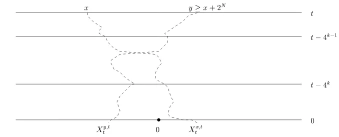
Figure 3: Illustration of the eventVkN.
the following t will be >> 22N. Let ∆t(s), for s < t, be the event that a crossing of two dual
coalescing random walks starting at timet(in the voter model) occurs in the dual time interval (s, t] and by the dual time t they are on opposite sides of the origin, i.e, there exists u, v ∈ Z
withXsu,t < Xsv,t and Xtv,t≤0< Xtu,t.
From the estimates in the proof of lemma 5 in Cox and Durrett [4], one can show that P(∆t(s))≤
C/√s, if we have that P(0∈ζs
s(Z))≤C/
√
s, which holds if p(·) has finite second moment (see Lemma5.6). Therefore, all we have to show is that
P {rt−lt≥2N} ∩(∆t(4N))c≤
C
2N (4.4)
for some C independent of t and N. We denote the event {rt−lt ≥2N} ∩(∆t(4N))c by VN
which is a subset of ∪N
k=0VkN where VkN is the event that (see Figure 3) there exists x, y ∈ Z
withy−x≥2N such that, for the coalescing walksXsx,t and Xsy,t,
(i) Xsx,t< Xsy,t for every 0≤s≤4k−1;
(ii) There existss∈(4k−1,4k] with Xsx,t > Xsy,t;
(iii) Xtx,t>0 and Xty,t≤0.
Fork= 0 we replace 4k−1 by 0. We will obtain suitable bounds on VkN which will enable us to conclude thatPN
k=0P(VkN)≤ 2CN.
Fix 0≤k≤N. For 0≤s≤tand y∈Z, we call
Ry(s) :=
supx∈Z{|x−y|:X
x,t
s =y} , if there exists x such thatXsx,t=y
0 , otherwise
therangeof the coalescing random walk at (s, y)∈(0, t]×Z. ObviouslyVN
k is contained in the
event that there existsx, y inζt
4k−1(Z) withx < y such that
(i) Rx(4k−1) +Ry(4k−1) +|y−x| ≥2N;
(ii) There existss∈(4k−1,4k] with Xsx,t−4−k4−k1−1 > X
y,t−4k−1
(iii) Xtx,t−4−k4−k1−1 >0,X
y,t−4k−1
t−4k−1 ≤0,
which we denote by ˜VkN.
We call the crossing between two coalescing random walks a relevant crossing if it satisfies conditions (i) and (ii) in the definition of ˜VkN up to the time of the crossing. We are interested in the density of relevant crossings between random walks in the time interval (4k−1,4k] and (as is also relevant) the size of the overshoot, i.e., the distance between the random walks just after crossing. To begin we consider separately three cases:
(i) The random walks at time 4k−1 are atx < y with|x−y| ≤2k−1 (so it is ”reasonable” to expect the random walks to cross in the time interval (4k−1,4k], and either R
x(4k−1) or
Ry(4k−1) must exceed 2N−2 ).
(ii) The random walks are separated at time 4k−1 by at least 2k−1 but no more than 2N−1 (so eitherRx(4k−1) or Ry(4k−1) must exceed 2N−2).
(iii) The random walks are separated at time 4k−1 by at least 2N−1. In this case we disregard the size of the range.
Before dealing specifically with each case, we shall consider estimates on the density of particles inζt
4k(Z) with range greater thanm2k. We first consider the density of random walks at time
4k which move by more thanm2k in the time interval (4k,4k+1]. By Lemma5.6, the density of
particles in ζ4tk(Z) is bounded by 2Ck. By the Markov property and Lemma 5.1, we obtain the
following result:
Lemma 4.3. For every 0 < β < 1, there exists c, C ∈ (0,∞) such that for every k ∈ N and m≥1, the probability that a fixed site y∈Zsatisfiesy∈ζt
4k(Z), and the backward random walk
starting at(y, t−4k) makes an excursion of size at leastm2k before reaching time level t−4k+1
is bounded by
C
2k
e−c(m2k)1−β +e−cm2 + 1
m3+ǫ2k(1+ǫ)
.
As a corollary, we have
Lemma 4.4. For every0< β <1, there existsc, C ∈(0,∞)so that for everyk∈Nandm≥1,
the density of y∈ζ2t2k(Z) whose range is greater than m2k is bounded by
C
2k
2ke−c(m2k)1−β +e−cm2 + 1
m3+ǫ2k(1+ǫ)
.
Proof:
Let dl,k be the density of coalescing random walks remaining at time 4l, which on interval
(4l,4l+1] move by more than
∞ X
r=1
1
r2
!−1 m2k
By Lemma4.3we have thatdl,k is bounded above by
C
2l
"
e−c
“ m2k (k−l)2
”1−β
+e
−c(m2k−l)2
(k−l)4 + (k−l)
2(3+ǫ)
(m2k−l)3+ǫ2l(1+ǫ)
#
.
It is not difficult to see thatP
l<kdl,k provides an upper bound for the density we seek. Summing
the above bounds fordl,k establishes the lemma.
We can now estimate the relevant crossing densities and overshoot size in cases (i), (ii) and (iii) above. More precisely, we will estimate the expectation of the overshoot between two random walks starting at x < y at time 4k−1 restricted to the event that: x, y ∈ζ4tk−1(Z), Rx and Ry
are compatible with y−x as stated in cases (i) –(iii), and the two walks cross before time 4k. From now on, we fixβ ∈(0,1).
Case (i): Since if the two events {x ∈ ζ4tk−1(Z)} ∩ {Rx(4k−1) > 2N−2} and {y ∈ ζ4tk−1(Z)}
both occur, they always occur on disjoint trajectories of random walks in the dual time interval [0,4k−1], we may apply the van den Berg-Kesten-Reimer inequality (see Lemma 4 in [2] and the discussion therein) which together with the previous lemma implies that the probability that
x, y∈ζt
4k−1(Z) and at least one has range 2N−2 is less than
C
4k
2ke−c2N(1−β) +e−c4N−k+ 4
k
2N(3+ǫ)
.
Moreover the expectation of the overshoot (see [4])
Xτx,t−4k−1 −Xτy,t−4k−1
on the eventτ ≤4k−4k−1= 3·4k−1 where
τ = inf{s >0 :Xsx,t−4k−1 −Xsy,t−4k−1 ≥0}
is the time of crossing, is uniformly bounded over kand y−x.
Case (ii): In this case we must also take into account that the probability of the two random walks crossing before time 4k is small. We analyze this by dividing up the crossing into two cases. In the first case the two random walks halve the distance between them before crossing. In the second case the crossing occurs due to a jump of order y−x.
Let
τ′ = inf
s >0 :Xsy,t−4k−1−Xsx,t−4k−1 < y−x
2
.
Then as in Case (i),
is uniformly bounded by some constantC >0. Therefore
EhXτx,t−4k−1 −Xτy,t−4k−1; τ′ < τ ≤3·4k−1; x, y∈ζ4tk−1(Z); Rx orRy ≥2N−2
i
≤C Pτ′<3·4k−1 Px, y∈ζ4tk−1(Z); Rx orRy ≥2N−2
≤C P x, y∈ζ4tk−1(Z); Rx orRy ≥2N−2
×
e−c|x−y|1−β +e−c(x−4ky)2 + 4
k
|x−y|3+ǫ
≤ C
4k
2ke−c2N(1−β)+e−c4N−k + 4
k
2N(3+ǫ)
×
e−c|x−y|1−β +e−c(x−4ky)2 + 4
k
|x−y|3+ǫ
.
On the other hand it is easily seen (by estimating the rates at which a large jump occurs, see Section3 for details) that
E[Xτx,t−4k−1 −Xτyt−4k−1, τ =τ′ <3·4k−1]≤C 4
k
|x−y|2+ǫ
and so we have a contribution
C
4k
2ke−c2(1−β)N+e−c4N−k + 4
k
2N(3+ǫ)
4k
|x−y|2+ǫ.
Case (iii): In this case we argue as in (ii) except the factor
2ke−c2(1−β)N+e−c4N−k + 4
k
2N(3+ǫ)
is dropped as we make no assumption on the size ofRx orRy. So our bound is
C
4k
4k
|x−y|2+ǫ +e
−c|x−y|1−β
+e−c(x−4ky)2 + 4
k
|x−y|(3+ǫ)
.
From the three cases above, we can sum over y ∈ Z and verify that, for a given site x ∈ Z,
the total expected overshoot associated with relevant crossings in the time interval (4k−1,4k] involving (x,4k−1) and (y,4k−1) for all possibley∈Z is bounded by
C 1
2N(1+ǫ) +e
−c2N(1−β)
+e
−c4N−k
2k
!
. (4.5)
We say a d-crossover (d∈ N) occurs at site x ∈ Z at time s ∈ (4k−1,4k] if at this time (dual
time, for coalescing random walks) a relevant crossing occurs leaving particles at sites x and
Ik(s, x, d). By translation invariance, the distribution of{Ik(s, x, d)}s∈(4k−1,4k]is independent of x∈Z.
LetXsx andXsx+dbe two independent random walks with transition probabilityp(·) starting at
x andx+dat time 0, and let τx,x+d= inf{s:Xsx=Xsx+d}. Then
invariance, it is not difficult to see that
X
x∈Z
PXtx−s≤0< Xtx−+sd, τx,x+d> t−s
=E[(Ztd−s)+, τ0 > t−s]≤Cd,
where the inequality withC >0 uniform over dandtis a standard result for random walks (see Lemma 2 in [4]).
Finally, to show (4.7), we note that the left hand side is the expected overshoot of relevant crossings where one of the two random walks after the crossing is at 0. By translation invariance this is bounded above by the expected overshoot associated with relevant crossings in the time interval (4k−1,4k] involving (0,4k−1) and (y,4k−1) for every y >0, which is estim ated in (4.5). Indeed, let Fk(x, y;m, m+d) be the indicator function of the event that a relevant crossover
a change of variable
4.3 Proof of (iii) in Theorem 1.4
We know from [1] that if γ ≥2, then the voter model interface evolves as a positive recurrent chain, and hence the equilibrium distributionπ exists. In particular,π{ξ0}>0 whereξ0 is the
trivial interface of the Heavyside configurationη1,0. Letξtdenote the interface configuration at
timetstarting with ξ0, and letν denote its distribution. Then
π{ξ : Γ(ξ)≥n}> π{ξ0}ν{Γ(ξt)≥n} (4.8)
LetXt2nandXt5ndenote the positions at timetof two independent random walks with transition probability p(·) starting at 2n and 5nat time 0. Let A denote the event that X2n
t ∈[n,3n] for
all t∈[0, n2], and let Bs, s∈ [0, n2], denote the event that Xt5n ∈[4n,6n] for all t∈[0, s) and
Xt5n∈(−∞,−n] for allt∈[s, n2]. EventBscan only occur ifXt5n makes a large negative jump
at times. By duality between voter models and coalescing random walks,
ν{Γ(ξn2)≥3n} ≥ P{ηn2(2n) = 0, ηn2(5n) = 1}
Condition on Xt5n staying inside [4n,6n] before time s and making a negative jump of size at least−8nat times, we have by the strong Markov property that
By Donsker’s invariance principle, the probability of each of the three events: A, \
which we may symmetrize to obtain
ν{Γ(ξn2)≥n} ≥ β
contradicting our assumption. This proves the first part of (iii) in Theorem1.4. To find random walk jump kernel p(·) satisfying (1.6), we can choose p(·) with P
|y|≥np(y) ∼ Cn−α for some
C >0. (1.6) then follows directly from (4.8) and (4.10).
5
Technical Estimates
The following lemmas for random walks will be needed.
Lemma 5.1. Let Xt be a centered continuous time one-dimensional random walk starting at
Proof: By the reflection principle for random walks, we only have to show that for every
for allM, T >0. To prove this inequality, we consider the following usual representation of Xt:
there exist centered i.i.d. random variables (Yn)n≥1onZwith finite 3 +ǫmoment and a Poisson
whereY0= 0. The analogue of (5.1) for discrete time random walks appears as corollary 1.8 in
[8], from which we obtain somec′, C′ >0. Then after adjusting the constants, we obtain
P(|XT| ≥M)≤C
We now suppose T ≤M. Back to the term after the first inequality in equation (5.3),
Lemma 5.2. Let Xtx and Xty be two independent identically distributed continuous time homo-geneous random walks with finite second moments starting from positions x and y at time 0. Let τx,y = inf{t >0 : Xtx =Xty} be the first meeting time of the two walks. Then there exists
C0>0 such that
P(τx,y > T)≤ √C0
T|x−y|
for allx, y and T >0.
Proof. This is a standard result. See, e.g., Proposition P4 in Section 32 of [10], or Lemma 2.2 of [9]. Both results are stated for discrete time random walks, but the continuous time analogue follows readily from a standard large deviation estimate for Poisson processes.
Lemma 5.3. Given a system of 2J coalescing random walks indexed by their starting positions
{x(1)1 , x(1)2 , ..., x1(J), x(2J)} at time 0, if
x1(1) < x(1)2 <· · ·< x(1i) < x2(i)<· · ·< x(1J) < x(2J),
andsupi|x(1i)−x2(i)| ≤M for some M >0, then for any fixed timeT > C02M2 withC0 satisfying Lemma 5.2, the number of coalesced walks by time T stochastically dominates the sum of J
independent Bernoulli random variables {Y1, ..., YJ}, each with parameter 1−C0M/
√
T. In particular
P(the number of coalesced particles by time T is smaller than N)
≤P
J
X
i=1
Yi≤N
!
.
Proof: To prove the lemma, we construct the system of coalescing random walks from the system of independent walks. Given the trajectories of a system of independent walks starting from positions{x(1)1 , x(1)2 , ..., x(1J), x(2J)}at time 0, the first time some walk, sayx(1i), jumps to the position of another walk, say x(2j), the walk x(1i) is consideredcoalesced, i.e., from that time on, it follows the same trajectory as walkx(2j), while the trajectory of walkx(2j) remains unchanged. Among the remaining distinct trajectories, we iterate this procedure until no more coalescing takes place. Note that this construction is well defined, since almost surely no two random walk jumps take place at the same time. The resulting collection of random walk trajectories is distributed as a system of coalescing random walks.
In the above construction, almost surely, the number of coalesced walks by time T in the coa-lescing system is bounded from below by the number of pairs{x(1i), x2(i)} (1≤i≤J) for which
x(1i) andx(2i)meet before timeT in the independent system. Ifx(1i)meetsx(2i)in the independent system at time t≤T, then in the coalescing system, either x1(i) and x(2i) haven’t coalescedwith other walks before timet, in which case the two will coalesce at time t; or one of the two walks has coalesced with another walk before time t. In either case, whenever x1(i) and x(2i) meet in the independent system, at least one of them will be coalesced in the coalescing system. The asserted stochastic domination then follows by noting that Lemma 5.2 implies that each pair
{x(1i), x2(i)} has probability at least 1−C0M/
√
Proposition 5.4. Let 12 < p <1be fixed. Consider a system of coalescing random walks starting with at mostγLparticles inside an interval of lengthL at time 0. LetK0 = 64C
2 0
(2p−1)4, whereC0 is
as in Lemma 5.2. If γL≥ 2p8−1, then there exist constants C, c depending only on p such that, the probability that the number of particles alive at timeT = K0
γ2 is greater than pγLis bounded
above byCe−cγL.
Proof: The basic idea is to apply Lemma5.3and large deviation bounds for Bernoulli random variables. The choice of the constantsK0 and T will become apparent in the proof.
Without loss of generality, we assumeγL∈N. We only need to consider a system starting with γLparticles. If the initial number of particles is less thanγL, we can always add extra particles to the system which only increases the probability of havingpγLparticles survive by time T. LetM be a positive integer to be determined later. Since the γLparticles partition the interval of length L into γL+ 1 pieces, the number of adjacent pairs of particles of distance at most
M−1 apart is at leastγL−1−ML. Therefore the number ofdisjointpairs of adjacent particles of distance at mostM−1 apart is at least 12(γL−2− L
M). Each such pair coalesces before time
T with probability at least 1−C0M/
√
T. By Lemma 5.3, the number of coalesced particles stochastically dominates the sum ofm:= 12(γL−2−ML) i.i.d. Bernoulli random variables with parameter 1−C0M/
√
T, which we denote byY1,· · ·, Ym. If by timeT, more thanpγLparticles
survive, then we must have
m
X
i=1
Yi ≤ (1−p)γL. (5.4)
Letp= 1+2ǫ withǫ∈(0,1), then we can rewrite (5.4) as
1
m
m
X
i=1
Yi ≤ 1 (1−p)γL
2(γL−2−ML)
= 1−ǫ
1−γL2 −γM1 . (5.5)
By our assumptionγL2 ≤ 14(2p−1) = 4ǫ. If we chooseM = ǫγ4, and letT = (2C0M
ǫ )2 =
64C2 0
ǫ4γ2 = Kγ20,
then we have
1
m
m
X
i=1
Yi ≤ 1−ǫ
1−ǫ/2 <1−C0M/
√
T = 1−ǫ/2.
By standard large deviation estimates for Bernoulli random variables with parameter 1−ǫ/2, the probability of the event in (5.4) is bounded above byCe−c′m for someC, c′ depending only on p. Since m = 12(γL−2− ML) ≥ (1/2−ǫ/4)γL by our choice of M and the assumption
γL ≥ 2p8−1, we have Ce−c′m
≤ Ce−c′(1/2−ǫ/4)γL
= Ce−cγL, which concludes the proof of the
lemma.
The next result allows us to carry out the first step in the chain argument of section2.
Lemma 5.5. In the system of backward coalescing random walks {Xx,s}
(x,s)∈Z×R dual to the