Asymptotic Expansions for Bounded Solutions
to Semilinear Fuchsian Equations
Xiaochun Liu and Ingo Witt
Received: Jun 12, 2002 Revised: July 15, 2004
Communicated by Bernold Fielder
Abstract. It is shown that bounded solutions to semilinear elliptic Fuchsian equations obey complete asymptotic expansions in terms of powers and logarithms in the distance to the boundary. For that pur-pose, Schulze’s notion of asymptotic type for conormal asymptotic ex-pansions near a conical point is refined. This in turn allows to perform explicit computations on asymptotic types — modulo the resolution of the spectral problem for determining the singular exponents in the asymptotic expansions.
2000 Mathematics Subject Classification: Primary: 35J70; Sec-ondary: 35B40, 35J60
Keywords and Phrases: Calculus of conormal symbols, conormal asymptotic expansions, discrete asymptotic types, weighted Sobolev spaces with discrete asymptotics, semilinear Fuchsian equations
Contents
1 Introduction 208
2 Asymptotic types 212
2.1 Fuchsian differential operators . . . 212
2.2 Definition of asymptotic types . . . 217
2.3 Pseudodifferential theory . . . 230
3 Applications to semilinear equations 238
3.1 Multiplicatively closed asymptotic types . . . 238 3.2 The bootstrapping argument . . . 244 3.3 Proof of the main theorem . . . 245 3.4 Example: The equation ∆u=Au2+B(x)uin three space dimensions 247
1 Introduction
In this paper, we study solutions u=u(x) to semilinear elliptic equations of the form
Au=F(x, B1u, . . . , BKu) onX◦=X\∂X. (1.1) Here, X is a smooth compact manifold with boundary,∂X, and of dimension
n+ 1, A, B1, . . . , BK are Fuchsian differential operators on X◦, see Defini-tion 2.1, with real-valued coefficients and of ordersµ,µ1, . . . , µK, respectively, where µJ < µ for 1≤J ≤K, and F =F(x, ν) :X◦×RK →R is a smooth function subject to further conditions as x→∂X. In caseA is elliptic in the sense of Definition 2.2 (a) we shall prove that bounded solutions u: X◦ → R
to Eq. (1.1) possess complete conormal asymptotic expansion of the form
u(t, y)∼
∞
X
j=0 mj
X
k=0
t−pjlogkt cjk(y) ast→+0. (1.2)
Here, (t, y) ∈[0,1)×Y are normal coordinates in a neighborhood U of ∂X,
Y is diffeomorphic to ∂X, and the exponents pj ∈ C appear in conjugated pairs, Repj → −∞ asj → ∞,mj ∈N, andcjk(y)∈C∞(Y). Note that such conormal asymptotic expansions are typical of solutions uto linear equations of the form (1.1), i.e., in caseF(x) =F(x, ν) is independent ofν∈RK. The general form (1.2) of asymptotics was first thoroughly investigated by
Kondrat’ev in his nowadays classical paper [9]. After that to assign asymp-totic types to conormal asympasymp-totic expansions of the form (1.2) has proved to be very fruitful. In its consequence, it provides a functional-analytic frame-work for treating singular problems, both linear and non-linear ones, of the kind (1.1). Function spaces with asymptotics will be discussed in Sections 2.4, 3.1. In its standard setting, going back to Rempel–Schulze [14] in case n = 0 (whenY is always assumed be a point) andSchulze[15] in the general case, an asymptotic typeP for conormal asymptotic expansions of the form (1.2) is given by a sequence {(pj, mj, Lj)}∞j=0, where pj ∈C, mj ∈N are as in (1.2), and Lj is a finite-dimensional linear subspace of C∞(Y) to which the coeffi-cientscjk(y) for 0≤k≤mj are required to belong. (In casen= 0, the spaces
When treating semilinear equations we shall encounter asymptotic types be-longing to bounded functionsu(x), i.e., asymptotic typesP for which
(
p0= 0,m0= 0,L0= span{1}, Repj<0 for allj≥1,
(1.3)
where 1∈L0 is the function onY being constant 1.
It turns out that this notion of asymptotic type resolves asymptotics not fine enough to suit a treatment of semilinear problems. The difficulty with it is that only the aspect of the production of asymptotics is emphasized — via the finite-dimensionality of the spacesLj— but not the aspect of their annihilation. For semilinear problems, however, the latter affair becomes crucial. Therefore, in Section 2, we shall introduce a refined notion of asymptotic type, where additionally linear relations between the various coefficientscjk(y)∈Lj, even for differentj, are taken into account.
Let As(Y) be the set of all these refined asymptotic types, while As♯(Y) ⊂ As(Y) denotes the set of asymptotic types belonging to bounded functions according to (1.3). ForR∈As(Y), letC∞
R(X) be the space of smooth functions
u∈C∞(X◦) having conormal asymptotic expansions of typeR, andC∞
R(X×
RK) =C∞(RK;CR∞(X)), whereCR∞(X) is equipped with its natural (nuclear) Fr´echet topology. In the formulation of Theorem 1.1, below, we will assume that F∈C∞
R(X×RK), where
ω(t)tµ−µ¯−εCR∞(X)⊂L∞(X) (1.4) for someε >0. Here, ¯µ= max1≤J≤KµJ< µandω=ω(t) is a cut-off function supported in U, i.e., ω ∈ C∞(X), suppω ⋐ U. Here and in the sequel, we
always assume that ω =ω(t) depends only on t for 0 < t <1 and ω(t) = 1 for 0 < t≤1/2. Condition (1.4) means that, given the operator A and then compared to the operators B1, . . . , BK, functions in CR∞(X) cannot be too singular ast→+0.
There is a small difference between the set Asb(Y) of all bounded asymptotic types and the set As♯(Y) of asymptotic types as described by (1.3); As♯(Y)(
Asb(Y). The set As♯(Y) actually appears as the set of multiplicatively closable asymptotic types, see Lemma 3.4. This shows up in the fact that when only boundedness is presumed asymptotic types belonging to Asb(Y) — but not to As♯(Y) — need to be excluded from the considerations by the following non-resonance type condition (1.5), below:
Let H−∞,δ(X) = S
s∈RHs,δ(X) for δ ∈ R be the space of distributions u =
u(x) on X◦ having conormal order at least δ. (The weighted Sobolev space
Hs,δ(X), wheres∈Ris Sobolev regularity, is introduced in (2.31).) Note that S
δ∈RH−∞,δ(X) is the space of all extendable distributions onX◦that in turn is dual to the spaceCO∞(X) of all smooth functions onX vanishing to infinite
Now, fixδ∈Rand suppose that a real-valuedu∈ H−∞,δ(X) satisfyingAu∈
C∞
O(X) has an asymptotic expansion of the form
u(x)∼Re
∞
X
j=0 mj
X
k=0
tl+j+iβlogkt cjk(y)
ast→+0,
where l∈Z, β ∈R,β 6= 0 (andl > δ−1/2 provided thatc0m0(y)6≡0 due to
the assumption u∈ H−∞,δ(X)). Then, for each 1≤J ≤K, it is additional required that
BJu=O(1) ast→+0 impliesBJu=o(1) ast→+0, (1.5) where O and o are Landau’s symbols. Condition (1.5) means that there is no real-valued u ∈ H−∞,δ(X) with Au ∈ C∞
O(X) such that BJu admits an asymptotic series starting with the term Re(tiβd(y)) for some β ∈ R\ {0},
d(y)∈C∞(Y). This condition is void ifδ≥1/2 + ¯µ.
Our main theorem states:
Theorem 1.1. Let δ ∈ R and A ∈ DiffµFuchs(X) be elliptic in the sense of
Definition 2.2 (a), BJ ∈DiffµFuchsJ (X) for1≤J ≤K, where µJ < µ, andF ∈
C∞
R(X ×Rk) for some asymptotic type R ∈As(Y) satisfying (1.4). Further,
let the non-resonance type condition (1.5) be satisfied. Then there exists an asymptotic type P ∈ As(Y) expressible in terms ofA, B1, . . . , BK, R, and δ
such that each solution u∈ H−∞,δ(X) to Eq. (1.1)satisfying B
Ju∈L∞(X)
for1≤J ≤K belongs to the spaceC∞
P (X).
Under the conditions of Theorem 1.1, interior elliptic regularity already implies
u∈C∞(X◦). Thus, the statement concerns the fact thatupossesses a
com-plete conormal asymptotic expansion of type P near ∂X. Furthermore, the asymptotic typeP can at least in principle be calculated onceA,B1, . . . , BK,
R, andδare known.
Some remarks about Theorem 1.1 are in order: First, the solution uis asked to belong to the space H−∞,δ(X). Thus, if the non-resonance type condition (1.5) is satisfied for allδ∈R— which is generically true — then the foregoing requirement can be replaced by the requirement for u being an extendable distribution. In this case, Pδ 4 Pδ′ for δ ≥ δ′ in the natural ordering of
asymptotic types, where Pδ denotes the asymptotic type associated with the conormal order δ. Moreover, jumps in this relation occur only for a discrete set of values ofδ∈Rand, generically, Pδ eventually stabilizes asδ→ −∞. Secondly, for a solution u ∈ C∞
Remark 1.2. Theorem 1.1 continues to hold for sectional solutions in vec-tor bundles over X. Let E0, E1, E2 be smooth vector bundles over X, A ∈ DiffµFuchs(X;E0, E1) be elliptic in the above sense, B ∈ DiffµFuchs−1 (X;E0, E2), and F ∈ C∞
R(X, E2;E1). Then, under the same technical assumptions as above, each solution uto Au=F(x, Bu) in the class of extendable distribu-tions withBu∈L∞(X;E
2) belongs to the spaceCP∞(X;E0) for some resulting asymptotic typeP.
Theorem 1.1 has actually been stated as one, though basic example for a more general method for deriving — and then justifying — conormal asymptotic expansions for solutions to semilinear elliptic Fuchsian equations. This method always works if one has boundedness assumptions as made above, but bound-edness can often successfully be replaced by structural assumptions on the nonlinearity. An example is provided in Section 3.4. The proposed method works indeed not only for elliptic Fuchsian equations, but for other Fuchsian equations as well. In technical terms, what counts is the invertible of the com-plete sequence of conormal symbols in the algebra of comcom-plete Mellin symbols under the Mellin translation product, and this is equivalent to the elliptic-ity of the principal conormal symbol (which, in fact, is a substitute for the non-characteristic boundary in boundary problems). For elliptic Fuchsian dif-ferential operator, this latter condition is always fulfilled.
The derivation of conormal asymptotic expansions for solutions to semilinear Fuchsian equations is a purely algebraic business once the singular exponents and their multiplicities for the linear part are known. However, a strict justifi-cation of these conormal asymptotic expansions — in the generality supplied in this paper — requires the introduction of the refined notion of asymptotic type and corresponding function spaces with asymptotics. For this reason, from a technical point of view the main result of this paper is Theorem 2.42 which states the existence of a complete sequence of holomorphic Mellin symbols realizing a given proper asymptotic type in the sense of exactly annihilating asymptotics of that given type. (The term “proper” is introduced in Defini-tion 2.22.) The construcDefini-tion of such Mellin symbols relies on the factorizaDefini-tion result of Witt[21].
Remark 1.3. Behind part of the linear theory, there is Schulze’s cone pseu-dodifferential calculus. The interested reader should consultSchulze[15, 16]. We do not go much into the details, since for most of the arguments this is not needed. Indeed, the algebra of complete Mellin symbols controls the pro-duction and annihilation of asymptotics, and it is this algebra that is detailed discussed.
difference between these two situations. Thus, the geometric situation is given by the kind of degeneracy admitted for, say, differential operators. In the case considered in this paper, this degeneracy is of Fuchsian type.
The first part of this paper, Section 2, is devoted to the linear theory and the introduction of the refined notion of asymptotic type. Then, in a second part, Theorem 1.1 is proved in Section 3.
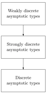
2 Asymptotic types
In this section, we introduce the notion of discrete asymptotic type. A compar-ison of this notion with the formerly known notions of weakly discrete asymp-totic type and strongly discrete asympasymp-totic type, respectively, can be found in Figure 1. The definition of discrete asymptotic type is modeled on part of the Gohberg-Sigal theory of the inversion of finitely meromorphic, operator-valued functions at a point, seeGohberg-Sigal[4]. See alsoWitt[18] for the corre-sponding notion of local asymptotic type, i.e., asymptotic types at one singular exponent p ∈ C in (1.2) only. Finally, in Section 2.4, function spaces with asymptotics are introduced. The definition of these function spaces relies on the existence of complete (holomorphic) Mellin symbols realizing a prescribed proper asymptotic type. The existence of such complete Mellin symbols is stated and proved in Theorem 2.42.
Added in proof. To keep this article of reasonable length, following the referee’s advice, proofs of Theorems 2.6, 2.30, and 2.42 and Propositions 2.28 (b), 2.31, 2.32, 2.35, 2.36, 2.40, 2.44, 2.46, 2.47, 2.48, 2.49, and 2.52 are only sketchy or missing at all. They are available from the second author’s homepage1.
2.1 Fuchsian differential operators
LetX be a compact C∞ manifold with boundary,∂X. Throughout, we fix a
collar neighborhoodU of∂X and a diffeomorphismχ:U →[0,1)×Y, withY
being a closed C∞ manifold diffeomorphic to∂X. Hence, we work in a fixed
splitting of coordinates (t, y) on U, where t ∈ [0,1) and y ∈Y. Let (τ, η) be the covariables to (t, y). The compressed covariable tτ to t is denoted by ˜τ, i.e., (˜τ , η) is the linear variable in the fiber of the compressed cotangent bundle
˜
T∗X¯¯
U. Finally, let dimX =n+ 1.
Definition 2.1. A differential operatorAwith smooth coefficients of orderµ
onX◦=X\∂X is called Fuchsian if
χ∗¡A
¯ ¯
U
¢ =t−µ
µ X
k=0
ak(t, y, Dy)¡−t∂t¢k, (2.1)
where ak ∈ C∞([0,1); Diffµ−k(Y)) for 0 ≤k ≤µ. The class of all Fuchsian differential operators of orderµonX◦is denoted by Diffµ
Weakly discrete asymptotic types
Singular exponents with multiplicities, (pj, mj), are prescribed, the coefficientscjk(y)∈C∞
(Y) are ar-bitrary. The general form of asymptotics is ob-served, cf., e.g., Kondrat’ev (1967), Melrose (1993),Schulze (1998).
❄
Strongly discrete asymptotic types
Singular exponents with multiplicities, (pj, mj), are prescribed,cjk(y)∈Lj⊂C
∞
(Y), where dimLj<
∞. The production of asymptotics is observed,
cf.Rempel–Schulze (1989),Schulze (1991).
❄
Discrete asymptotic types
Linear relation between the various coefficients
cjk(y)∈Lj, even for differentj, are additionally al-lowed. Thus theproduction/annihilation of asymp-totics is observed, cf. this article.
Figure 1: Schematic overview of asymptotic types
Henceforth, we shall suppress writing the restriction·¯¯Uand the operator push-forwardχ∗ in expressions like (2.1). ForA∈DiffµFuchs(X), we denote by
σµψ(A)(t, y, τ, η) =t−µ
µ X
k=0
σψµ−k(ak(t))(y, η)(itτ)k
the principal symbol ofA, by ˜σψµ(A)(t, y,τ , η˜ ) its compressed principal symbol related toσµψ(A)(t, y, τ, η) via
σψµ(A)(t, y, τ, η) =t−µσ˜µ
ψ(A)(t, y, tτ, η) in ( ˜T∗X\0)¯¯
U, and byσ
µ
M(A)(z) itsprincipal conormal symbol,
σMµ(A)(z) = µ X
k=0
ak(0)zk, z∈C.
Further, we introduce thejth conormal symbol σMµ−j(A)(z) forj = 1,2, . . . by
σMµ−j(A)(z) = µ X
k=0 1
j!
∂ja k
∂tj (0)z
k, z∈C.
ifA∈DiffµFuchs(X),B∈DiffFuchsν (X), thenAB∈DiffµFuchs+ν (X),
σMµ+ν−l(AB)(z) = X j+k=l
σMµ−j(A)(z+ν−k)σMν−k(B)(z) (2.2)
for alll= 0,1,2, . . . This formula is called theMellin translation product (due to the shifts ofν−k in the argument of the first factors).
Definition2.2. (a) The operator A∈DiffµFuchs(X) is calledelliptic ifAis an elliptic differential operator onX◦and
˜
σµψ(A)(t, y,τ , η˜ )6= 0, (t, y,τ , η˜ )∈( ˜T∗X\0)¯¯
U. (2.3)
(b) The operator A∈DiffµFuchs(X) is called elliptic with respect to the weight
δ∈RifAis elliptic in the sense of (a) and, in addition,
σµM(A)(z) :Hs(Y)→Hs−µ(Y), z∈Γ(n+1)/2−δ, (2.4) is invertible for somes∈R(and then for alls∈R). Here, Γβ={z∈C; Rez=
β} forβ∈R.
Under the assumption of interior ellipticity of A, (2.3) can be reformulated as µ
X
k=0
σµψ−k(ak(0))(y, η) ¡
iτ˜¢k 6= 0
for all (0, y,τ , η˜ )∈( ˜T∗X\0)¯¯
∂U. This relation implies thatσ
µ M(A)(z)
¯ ¯Γ
(n+1)/2−δ
is parameter-dependent elliptic as an element inLµcl¡Y; Γ(n+1)/2−δ ¢
, where the latter is the space ofclassical pseudodifferential operators onY of orderµwith parameterz varying in Γ(n+1)/2−δ, for
σµψ(σMµ (A))(y, z, η)¯¯z=(n+1)/2−δ−τ˜= ˜σψµ(A)(0, y,τ , η˜ ),
where σµψ(·) on the left-hand side denotes the parameter-dependent principal symbol. Thus, if (a) is fulfilled, then it follows that σµM(A)(z) in (2.4) is invertible forz∈Γ(n+1)/2−δ,|z|large enough.
Lemma 2.3. If A ∈ DiffµFuchs(X) is elliptic, then there exists a discrete set D ⊂ Cwith D ∩ {z∈C;c0 ≤Rez≤c1} is finite for all−∞< c0< c1 <∞
such that (2.4)is invertible for all z∈C\ D. In particular, there is a discrete setD⊂Rsuch thatA is elliptic with respect to the weightδfor allδ∈R\D;
D= ReD.
Proof. Since σMµ(A)(z)¯¯Γ
β ∈L
µ(Y; Γβ) is parameter-dependent elliptic for all
Next, we introduce the class of meromorphic functions arising in point-wise inverting parameter-dependent elliptic conormal symbols σµM(A)(z). The fol-lowing definition is taken from Schulze[16, Definition 2.3.48]:
Definition2.4. (a)MµO(Y) forµ∈Z∪ {−∞}is the space of all holomorphic functionsf(z) onCtaking values inLµcl(Y) such thatf(z)¯¯z=β+iτ ∈Lµcl(Y;Rτ) uniformly inβ∈[β0, β1] for all−∞< β0< β1<∞.
(b)M−∞
as (Y) is the space of all meromorphic functionsf(z) onCtaking values in L−∞(Y) that satisfy the following conditions:
(i) The Laurent expansion around each polez=poff(z) has the form
as(Y) is a filtered algebra under pointwise multiplication. For f ∈ Mµ
as(Y) for µ ∈ Z and f(z) = f0(z) +f1(z), where f0 ∈ MµO(Y),
f1 ∈ M−∞as (Y), the parameter-dependent principal symbolσ µ is independent of the choice of the decomposition off and also independent of
β ∈R. It is called the principal symbol off. The Mellin symbolf ∈ Mµ as(Y) is called ellipticif its principal symbol is everywhere invertible.
For the next result, seeSchulze[16, Theorem 2.4.20]:
Proposition 2.5. The Mellin symbol f ∈ Mµ
as(Y) for µ ∈ Z is invertible
In various constructions, it is important to have examples of elliptic Mellin symbolsf ∈ Mµ
Theorem 2.6. Let µ∈Zand{pj}j=1,2,... ⊂Cbe a sequence obeying the
prop-erty mentioned in Definition 2.4 (b) (ii). Let, for eachj = 1,2, . . ., operators
f−jνj, . . . , f
j Nj inL
µ
cl(Y), where νj≥0,Nj+νj≥0, be given such that • f−jνj, . . . , f
j
min{Nj,0}∈L
−∞(Y)are finite-rank operators,
• there is an ellipticg∈ MµO(Y)such that, for allj,0≤k≤Nj,
fkj− 1
k!g
(k)(pj)∈L−∞(Y) (2.7)
(in particular, fkj ∈Lµcl−k(Y) for0≤k≤Nj andf0j ∈L µ
cl(Y)is elliptic
of index zero).
Then there is an elliptic Mellin symbol f(z)∈ Mµ
as(Y)such that, for all j,
[f(z)]Nj
pj =
f−jνj
(z−pj)νj +· · ·+
f−j1
z−pj +f j
0+· · ·+f j
Nj(z−pj)
Nj, (2.8)
whilef(q)∈Lµcl(Y)is invertible for allq∈C\Sj=1,2,...{pj}.
Ifn= 0, condition (2.7) is void. In casen >0, however, this condition expresses several compatibility conditions among the σµψ−l(fkj), where j = 0,1,2, . . ., 0≤k≤Nj, andl≥k, and also certain topological obstructions that must be fulfilled. For instance, for anyf ∈ MµO(Y),
σψµ−j(f(z))(y, η) = j X
k=0
(z−p)k
k! σ µ−j ψ (f
(k)(p))(y, η), j= 0,1,2, . . .
in local coordinates (y, η) — showing, among others, that σψµ−j(f(z)) is poly-nomial of degreej with respect toz∈C. The point is that we do not assume
g(q)∈Lµcl(Y) be invertible forq∈C\ S
j=1,2,...{pj}.
Proof of Theorem 2.6. This can be proved using the results of Witt[21]. In particular, the factorization result there gives directly the existence of f(z) if the sequence{pj} ⊂Cis void.
Now, we are going to introduce the basic object of study — the algebra of complete conormal symbols. This algebra will enable us to introduce the refined notion of asymptotic type and to study the behavior of conormal asymptotics under the action of Fuchsian differential operators.
Definition 2.7. (a) Forµ∈Z, the space SymbµM(Y) consists of all sequences Sµ={sµ−j(z);j∈N} ⊂ Mµas(Y).
(b) An element Sµ ∈ Symbµ
M(Y) is called holomorphic if Sµ = {sµ−j(z);
(c)Sµ∈ZSymb µ
M(Y) is a filtered algebra under theMellin translation product, denoted by ♯M. Namely, for Sµ = {sµ−j(z); j ∈ N} ∈ SymbµM(Y), Tν = {tν−k(z);k ∈ N} ∈ SymbνM(Y), we define Uµ+ν =Sµ♯MTν ∈ Symbµ+ν
M (Y), whereUµ+ν={uµ+ν−l(z);l∈N}, by
uµ+ν−l(z) = X j+k=l
sµ−j(z+ν−k)tν−k(z) (2.9)
forl= 0,1,2, . . . See also (2.2).
From Proposition 2.5, we immediately get:
Lemma 2.8. Sµ ={sµ−j(z);j ∈N} ∈Symbµ
M(Y)is invertible in the filtered
algebra Sµ∈ZSymb µ
M(Y) if and only ifsµ(z)∈ Mµas(Y) is elliptic. In the case of the preceding lemma, Sµ ∈ Symbµ
M(Y) is called elliptic. A holomorphic elliptic Sµ ∈ Symbµ
M(Y) is called elliptic with respect to the weight δ ∈ Rif the line Γ(n+1)/2−δ is free of poles of sµ(z)−1. Notice that a holomorphic elliptic Sµ ∈ Symbµ
M(Y) is elliptic for all, but a discrete set of
δ ∈ R. The inverse to Sµ with respect to the Mellin translation product is denoted by (Sµ)−1. The set of elliptic elements of Symbµ
M(Y) is denoted by Ell SymbµM(Y).
There is a homomorphism of filtered algebras, [
µ∈N
DiffµFuchs(X)→ [ µ∈Z
SymbMµ (Y), A7→©σMµ−j(A)(z);j∈Nª.
By the remark preceding Lemma 2.3, ©σµM−j(A)(z);j ∈ Nª ∈ SymbµM(Y) is elliptic ifA∈DiffFuchs(X) is elliptic in the sense of Definition 2.2 (a).
2.2 Definition of asymptotic types
We now start to introduce discrete asymptotic types.
2.2.1 The spaces Eδ(Y) andEV(Y)
Here, we construct the “coefficient” space Eδ(Y) =S
V∈CδEV(Y) that admits
the non-canonical isomorphism (2.13), below,
Cas∞,δ(X) ±
CO∞(X) ∼=
−→ Eδ(Y),
where C∞,δ
as (X) is the space of smooth functions on X◦ obeying conormal
asymptotic expansions of the form (1.2) of conormal order at least δ, i.e., Repj < (n+ 1)/2−δ holds for all j (with the condition that the singular exponentspj appear in conjugated pairs dropped), andCO∞(X) is the subspace
Definition2.9. AcarrierV of asymptoticsfor distributions of conormal order
δis a discrete subset ofCcontained in the half-space{z∈C; Rez <(n+1)/2−
δ} such that, for all β0, β1 ∈R, β0 < β1, the intersection V ∩ {z ∈ C;β0 < Rez < β1}is finite. The set of all these carriers is denoted byCδ.
In particular,Vp=p−Nforp∈Cis such a carrier of asymptotics. Note that
Vp∈ Cδ if and only if Rep <(n+ 1)/2−δ. We setT̺V =̺+V ∈ C−̺+δ for
̺∈RandV ∈ Cδ. We further setC=S δ∈RCδ. Let [C∞(Y)]∞ = Sm∈N[C
∞(Y)]m be the space of all finite sequences in
C∞(Y), where the sequences (φ
0, . . . , φm−1) and (0, . . . ,0 | {z } htimes
, φ0, . . . , φm−1) for
h ∈ N are identified. For V ∈ Cδ, we set EV(Y) = Q
p∈V[C∞(Y)]∞p , where [C∞(Y)]∞
p is an isomorphic copy of [C∞(Y)]∞, and define Eδ(Y) to be the space of all families Φ ∈ EV(Y) for some V ∈ Cδ depending on Φ. Thereby, Φ ∈ EV(Y), Φ′ ∈ EV′(Y) for possibly different V, V′ ∈ Cδ are identified if Φ(p) = Φ′(p) for p ∈ V ∩V′, while Φ(p) = 0 for p∈ V \V′, Φ′(p) = 0 for
p∈V′\V. Under this identification,
Eδ(Y) = [ V∈Cδ
EV(Y). (2.10)
Moreover,EV(Y)∩ EV′(Y) =EV∩V′(Y).
On [C∞(Y)]∞, we define theright shift operator T by
(φ0, . . . , φm−2, φm−1)7→(φ0, . . . , φm−2).
On Eδ(Y), the right shift operator T acts component-wise, i.e., (TΦ)(p) =
T(Φ(p)) for Φ∈ EV(Y) and allp∈V.
Remark 2.10. To designate different shift operators with the same symbolT, once T̺ for̺ ∈R for carriers of asymptotics, once T, T2, etc. for vectors in Eδ(Y) should not confuse the reader.
For Φ ∈ Eδ(Y), we define c-ord(Φ) = (n+ 1)/2−max{Rep; Φ(p) 6= 0}. In particular, c-ord(0) = ∞. Note that c-ord(Φ) > δ if Φ ∈ Eδ(Y). For Φi ∈ Eδ(Y),α
i∈Cfori= 1,2, . . . satisfying c-ord(Φi)→ ∞asi→ ∞, the sum Φ =
∞
X
i=1
αiΦi, (2.11)
is defined in Eδ(Y) in an obvious fashion: Let Φi ∈ EV
i(Y), where Vi ∈ C
δi,
δi ≥ δ, and δi → ∞ as i → ∞. Then V = SiVi ∈ Cδ, and Φ ∈ EV(Y) is defined by Φ(p) =P∞i=1αiΦi(p) forp∈V, where, for eachp∈V, the sum on the right-hand side is finite.
Lemma2.11. LetΦi ∈ Eδ(Y)fori= 1,2, . . .,c-ord(Φi)→ ∞asi→ ∞. Then
(2.11) holds if and only if
c-ord(Φ− N X
i=1
Note that (2.12) already implies that c-ord(αiΦi)→ ∞asi→ ∞.
Definition 2.12. Let Φi, i= 1,2, . . ., be a sequence inEδ(Y) with the prop-erty that c-ord(Φi) → ∞ as i → ∞. Then this sequence is called linearly independent if, for allαi∈C,
∞
X
i=1
αiΦi= 0
implies thatαi= 0 for alli. A linearly independent sequence Φifori= 1,2, . . . inJfor a linear subspaceJ⊆ Eδ(Y) is called abasisforJ if every vector Φ∈J can be represented in the form (2.11) with certain (then uniquely determined) coefficientsαi ∈C.
Note that P∞i=1αiΦi = 0 in Eδ(Y) if and only if c-ord(PN
i=1αiΦi) → ∞ as
N → ∞according to Lemma 2.11. We also obtain:
Lemma 2.13. Let Φi, i = 1,2, . . ., be a sequence in Eδ(Y) such that c-ord(Φi) → ∞ as i → ∞. Further, let {δj}∞j=1 be a strictly increasing
se-quence such that δj > δ for all j and δj → ∞ as j → ∞. Assume that the Φi are numbered in such a way that c-ord(Φi)≤δj if and only if 1≤i≤ej.
Then the sequence Φi, i = 1,2, . . ., is linearly independent provided that, for each j= 1,2, . . .,
Φ1, . . . ,Φej are linearly independent over the spaceE
δj(Y).
We now introduce the notion of characteristic basis:
Definition 2.14. Let J ⊆ Eδ(Y) be a linear subspace, T J ⊆ J, and Φi for
i= 1,2, . . . be a sequence inJ. Then Φi,i= 1,2, . . ., is called acharacteristic basis ofJ if there are numbersmi ∈N∪ {∞}such thatTmiΦi= 0 ifmi <∞, while the sequence{TkΦi;i= 1,2, . . . ,0≤k < mi} forms a basis forJ.
Remark 2.15. This notion generalizes a notion of Witt [18]: There, given a finite-dimensional linear space J and a nilpotent operator T: J → J, the sequence Φ1, . . . ,ΦeinJ has been called acharacteristic basis, of characteristic (m1, . . . , me), if
Φ1, TΦ1, . . . , Tm1−1Φ1, . . . ,Φe, TΦe, . . . , Tme−1Φe,
constitutes a Jordan basis ofJ. The numbersm1, . . . , meappear as the sizes of Jordan blocks; dimJ =m1+· · ·+me. The tuple (m1, . . . , me) is also called the
characteristicofJ(with respect toT),eis called thelengthof its characteristic, and Φ1, . . . ,Φe is sometimes said to be a an (m1, . . . , me)-characteristic basis ofJ. The space{0} has empty characteristic of lengthe= 0.
The question of the existence of a characteristic basis obeying one more special property is taken up in Proposition 2.20.
Definition 2.16. Φ∈ Eδ(Y) is called aspecial vector if Φ∈ Eδ
Vp(Y) for some
p∈C.
Thus, Φ∈ EV(Y) is a special vector if there is ap∈C, Rep <(n+1)/2−δsuch that Φ(p′) = 0 for allp′∈V,p′ ∈/ p−N. Obviously, if Φ6= 0, thenpis uniquely
determined by Φ, by the additional requirement that Φ(p)6= 0. We denote this complex numberpbyγ(Φ). In particular, c-ord(Φ) = (n+ 1)/2−Reγ(Φ).
2.2.2 First properties of asymptotic types
In the sequel, we fix a splitting of coordinates U →[0,1)×Y, x7→(t, y), near
∂X. Then we have the non-canonical isomorphism
Cas∞,δ(X) ±
CO∞(X) ∼=
−→ Eδ(Y), (2.13)
assigning to eachformal asymptotic expansion
u(x)∼X p∈V
X
k+l=mp−1 (−1)k
k! t
−plogkt φ(p)
l (y) ast→+0 (2.14)
for some V ∈ Cδ,m
p∈N, the vector Φ∈ EV(Y) given by
Φ(p) = (¡
φ0(p), φ(1p), . . . , φm(p)p−1¢ ifp∈V,
0 otherwise,
see also (2.30). “Non-canonical” in (2.13) means that the isomorphism depends explicitly on the chosen splitting of coordinatesU →[0,1)×Y,x7→(t, y), near
∂X. Coordinate invariance is discussed in Proposition 2.32.
Note the shift frommptomp−1 that for notational convenience has appeared in formula (2.14) compared to formula (1.2).
Definition 2.17. An asymptotic type, P, for distributions as x → ∂X, of conormal order at leastδ,is represented— in the given splitting of coordinates near ∂X — by a linear subspace J ⊂ EV(Y) for some V ∈ Cδ such that the following three conditions are met:
(a)T J ⊆J.
(b) dimJδ+j <∞for allj∈N, whereJδ+j =J/(J∩ Eδ+j(Y)). (c) There is a sequence{pj}M
j=1⊂C, whereM ∈N∪{∞}, Repj <(n+1)/2−δ, and Repj→ −∞asj → ∞ifM =∞, such thatV ⊆SMj=1Vpj and
J = M M
j=1 ³
J∩ EVpj(Y)´. (2.15)
Definition 2.18. Letu∈C∞,δ
Thus, by representation of an asymptotic type it is meant that P that — in the philosophy of asymptotic algebras, see Witt [20] — is the same as the linear subspace C∞ namelyT̺P is represented by the space
T̺J =©Φ∈ E̺+δ thus,Jpis a local asymptotic type in the sense of Witt[18].
commutes and the action ofT onJ is that one induced by (2.18), (2.19).
Proposition2.19. LetJ ⊂ EV(Y)be a linear subspace for someV ∈ Cδ. Then
there is a sequence Φi for i= 1,2, . . . of special vectors with c-ord(Φi)→ ∞
as i→ ∞ such that the vectorsTkΦi fori= 1,2, . . .,k= 0,1,2. . . span J if
and only ifJ fulfills conditions (a),(b), and (c).
In the situation just described, we writeJ =hΦ1,Φ2, . . .i.
Proof. LetJ ⊂ EV(Y) fulfill conditions (a) to (c). Due to (c) we may assume that V =Vp for somep∈C. Suppose that the special vectors Φ1, . . . ,Φe∈J have already been chosen (wheree= 0 is possible). Then we choose the vector Φe+1 among the special vectors Φ ∈ J which do not belong to hΦ1, . . . ,Φei such that Reγ(Φe+1) is minimal. We claim that J =hΦ1,Φ2, . . .i. In fact, c-ord(Φi) = (n+ 1)/2−Reγ(Φi)→ ∞ as i→ ∞ and, if Φ is a special vector in J, then Φ∈ hΦ1, . . . ,Φei, where eis such that Reγ(Φe)≤Reγ(Φ), while Reγ(Φe+1) > Reγ(Φ). Otherwise, Φe+1 would not have been chosen in the (e+ 1)th step.
The other direction is obvious.
For j ≥ 1, let (mj1, . . . , mjej) denote the characteristic of the space J
δ+j, see Remark 2.15
Proposition 2.20. Let J ⊂ EV(Y) be a linear subspace and assume that the special vectors Φi for i = 1,2, . . . , e, where e ∈ N∪ {∞}, as constructed in
Proposition 2.19, form a characteristic basis of J. Then the following condi-tions are equivalent:
(a) For each j, ΠjΦ1, . . . ,ΠjΦjej is an (m
j
1, . . . , mjej)-characteristic basis of
Jδ+j;
(b) For each j, Tmj1−1Φ
1, . . . , Tmej−1Φej are linearly independent over the
spaceEδ+j(Y), whileTkΦi∈ Eδ+j(Y)if either1≤i≤e
j,k≥mji ori > ej.
In particular, if (a), (b)are fulfilled, then, for anyj′ > j,Πjj′Φj′
1, . . . ,Πjj′Φj ′
ej
is a characteristic basis of Jδ+j, while Πjj′Φj′
ej+1 =· · ·= Πjj′Φ
j′
e′
j = 0. Here,
Φji′= Πj′Φi for1≤i≤ej′.
Proof. This is a consequence of Lemma 2.13 andWitt[18, Lemma 3.8]. Notice that, for a linear subspace J ⊂ EV(Y) satisfying conditions (a) to (c) of Definition 2.17, a characteristic basis possessing the equivalent properties of Proposition 2.20 need not exist. We provide an example:
Example 2.21. Let the spaceJ =hΦ1,Φ2i ⊂ EVp(Y) for somep∈C, Rep <
| {z } Φ1
| {z }
Φ2
p−1 p p−1 p
ψ1
⋆
⋆
ψ0
⋆
ψ1
⋆
Figure 2: Example of a non-proper asymptotic type
Π2Φ1, TΠ2Φ1−Π2Φ2 is a (3,1)-characteristic basis of Jδ+2, and any other characteristic basis ofJδ+2 is, up to a non-zero multiplicative constant, of the
form (
Π2Φ1+α1TΠ2Φ1+α2T2Π2Φ1+α3Π2Φ2,
β1(TΠ2Φ1−Π2Φ2) +β2T2Π2Φ1,
(2.20)
where α1, α2, α3, β1, β2 ∈Cand β16= 0. But then the conclusion in Propo-sition 2.20 is violated, since both vectors in (2.20) have non-zero image under the projection Π12, while Π1Φ1is a (2)-characteristic basis of Jδ+1.
Definition 2.22. An asymptotic type P ∈ Asδ(Y) represented by the lin-ear subspace J ⊂ EV(Y) is called proper if J admits a characteristic basis Φ1,Φ2, . . . satisfying the equivalent conditions in Proposition 2.20. The set of all proper asymptotic types is denoted by Asδprop(Y)(Asδ(Y).
For Φ∈ Eδ(Y),p∈C, and Φ(p) = (φ(p) 0 , φ
(p) 1 , . . . , φ
(p)
mp−1) we shall use, for any
q∈C, the notation
Φ(p)[z−q] = φ (p) 0 (z−q)mp +
φ(1p)
(z−q)mp−1 +· · ·+
φ(mp)p−1
z−q ∈ Mq(C
∞(Y)),
where Mq(C∞(Y)) is the space of germs of meromorphic functions at z =q
taking values in C∞(Y). Analogously, Aq(C∞(Y)) is the space of germs of
holomorphic functions atz=ptaking values inC∞(Y).
Definition 2.23. For Sµ ={sµ−j(z);j ∈N} ∈Symbµ
M(Y), the linear space
Lδ
Sµ ⊆Cas∞,δ(X)
±
C∞
O(X) is represented by the space of Φ∈ Eδ(Y) for which
there are functionsφe(p)(z)∈ Ap(C∞(Y)) forp∈C, Rep <(n+ 1)/2−δ, such
that
[(n+1)/2−δ+µ−Req]−
X
j=0
sµ−j(z−µ+j) µ
Φ(q−µ+j)[z−q]
+ φe(q−µ+j)(z−µ+j) 
for all q ∈ C, Req < (n+ 1)/2−δ+µ. Here, [a]− for a ∈ R is the largest
integer strictly less thana, i.e., [a]−∈Zand [a]− < a≤[a]−+ 1.
Remark 2.24. (a) If Φ∈ EV(Y) for V ∈ Cδ, then condition (2.21) is effective only if
q∈
[(n+1)/2−δ+µ−Req]−
[
j=0
Tµ−jV.
(b) If Φ∈ Eδ(Y) belongs to the representing space ofLδ
Sµ, and ifu∈Cas∞,δ(X)
possesses asymptotics given by the vector Φ according to (2.16), then there is a v∈C∞
O(X) such that ∞
X
j=0
ω(cjt)t−µ+jop(Mn+1)/2−δ
¡sµ−j(z)¢ω˜(c
jt) (u+v)∈CO∞(X).
Here, the numbers cj >0 are chosen so that cj → ∞ as j → ∞ sufficiently fast so that the infinite sum converges. For the notation op(Mn+1)/2−δ(. . .) see (2.35), below.
Definition2.25. ForP∈Asδ(Y) being represented byJ ⊂ EV(Y) andSµ∈ SymbµM(Y), thepush-forward Qδ−µ(P;Sµ) of P under Sµ is the asymptotic type in Asδ−µ(Y) represented by the linear subspaceK⊂ ET−µV(Y) consisting
of all vectors Ψ∈ ET−µV(Y) such that there is a Φ∈J and there are functions
e
φ(p)(z)∈ Ap(C∞(Y)) forp∈V such that
Ψ(q)[z−q] =
[(n+1)/2−δ+µ−Req]−
X
j=0 h
sµ−j(z−µ+j)³Φ(q−µ+j)[z−q] +φe(q−µ+j)(z−µ+j)´i
∗
q, (2.22) holds for allq∈TµV, see (2.6).
Remark 2.26. For aholomorphic Sµ ∈Symbµ
M(Y), one needs not to refer to the holomorphic functionsφe(p)(z)∈ Ap(C∞(Y)) forp∈V in order to define
the push-forwardQδ−µ(P;Sµ) in (2.22). We then also writeQ(P;Sµ) instead ofQδ−µ(P;Sµ).
Extending the notion of push-forward from asymptotic types to arbitrary linear subspaces ofC∞,δ
as (X) ±
C∞
O(X), the spaceLδSµ ⊆Cas∞,δ(X)
±
C∞
O(X) forSµ∈
SymbµM(Y) appears as the largest subspace ofC∞,δ as (X)
±
C∞
O(X) for which
Qδ−µ(LδSµ;Sµ) =Qδ−µ(O;Sµ). (2.23)
In this sense, it characterizes theamount of asymptotics of conormal order at leastδannihilated by Sµ∈Symbµ
Definition 2.27. A partial ordering on Asδ(Y) is defined by P 4 P′ for
P, P′∈Asδ(Y) if and only ifJ ⊆J′, whereJ, J′⊂ Eδ(Y) are the representing spaces forP andP′, respectively.
Proposition 2.28. (a) The p.o. set (Asδ(Y),4) is a lattice in which each non-empty subset S admits a meet, VS, represented by TP∈SJP, and each
bounded subset T admits a join, WT, represented by PQ∈T JQ, where JP
and JQ represent the asymptotic types P and Q, respectively. In particular, V
Asδ(Y) =O.
(b)ForP ∈Asδ(Y),Sµ∈Symbµ
M(Y), we haveQδ−µ(P;Sµ)∈As
δ−µ(Y).
Proof. (a) is immediate from the definition of asymptotic type and (b) can be checked directly on the level of (2.22).
Remark 2.29. Each element Sµ ∈ Symbµ
M(Y) induces a natural action
C∞,δ
as (X) → Cas∞,δ(X) ±
C∞
O(X). Its expression in the splitting of coordinates
U →[0,1)×Y,x7→(t, y), is given by (2.22).
In the language of Witt [20], this means that the quadruple ¡S
µ∈ZSymb µ
M(Y), Cas∞,δ(X), CO∞(X),As
δ(Y)¢is an
asymptotic algebra that is evenreduced; thus providing justification for the above choice of the notion of asymptotic type.
Theorem 2.30. For a holomorphic Sµ ∈ Ell Symbµ
M(Y), we have LδSµ ∈
Asδprop(Y).
Proof. LetSµ ={sµ−j(z);j ∈N} ⊂ Mµ
O(Y). Assume that, for some p∈C,
Rep < (n+ 1)/2−δ, Φ0 ∈ Lsµ(z) at z = p, with the obvious meaning, for
this see Witt [18]. (Notice that Lsµ(z) at z = p is contained in the space
[C∞(Y)]∞.) We then successively calculate the sequence Φ
0,Φ1,Φ2, . . . from the relations, atz=p,
sµ(z−j)Φj[z−p] +sµ−1(z−j+ 1)Φj−1[z−p]
+· · ·+sµ−j(z)Φ0[z−p]∈ Ap(C∞(Y)), j= 0,1,2, . . . , (2.24) see (2.22) and Remark 2.26. In each step, we find Φj ∈ [C∞(Y)]∞ uniquely
determined moduloLsµ(z) atz=p−j such that (2.24) holds. We obtain the
vector Φ∈ EVp(Y) define by Φ(p−j) = Φj that belongs to the linear subspace
J ⊂ Eδ(Y) representing Lδ
Sµ.
Conversely, each vector in J is a sum like in (2.11) of vectors Φ obtained in that way. Thus, upon choosing in each space Lsµ(z) at z =p a characteristic
basis and then, for each characteristic basis vector Φ0 ∈ [C∞(Y)]∞, exactly one vector Φ∈ EVp(Y) as just constructed, we obtain a characteristic basis of
J in the sense of Definition 2.14 consisting completely of special vectors (since
Lsµ(z) atz =pequals zero for allp∈C, Rep <(n+ 1)/2−δ, but a set of p
belonging to Cδ). In particular,J ⊂ EV(Y) for someV ∈ Cδ and (a) to (c) of Definition 2.17 are satisfied. By its very construction, this characteristic basis fulfills condition (b) of Proposition 2.20. Therefore, the asymptotic typeLδ
Sµ
In conclusion, we obtain:
Proposition2.31. Let Sµ∈Ell Symbµ
M(Y). Then: (a) Lδ
Sµ =Qδ(O; (Sµ)−1)andL
δ−µ
(Sµ)−1 =Qδ−µ(O;Sµ).
(b)There is an order-preserving bijection
©
P ∈Asδ(Y);P <LδSµ
ª
→©Q∈Asδ−µ(Y);Q<Lδ(S−µµ)−1
ª
, (2.25)
P 7→ Qδ−µ(P;Sµ),
with the inverse given byQ7→ Qδ(Q; (Sµ)−1).
Proof. Using Proposition 2.28 (b), the proof consists of a word-by-word repeti-tion of the arguments given in the proof of Witt[18, Proposition 2.5]. In its consequence, Proposition 2.31 enables one to perform explicit calculations on asymptotic types.
We conclude this section with the following basic observation:
Proposition 2.32. The notion of asymptotic type, as introduced above, is invariant under coordinates changes.
Proof. Let κ: X → X be a C∞ diffeomorphism and let κ
∗: C∞(X◦) →
C∞(X◦) be the corresponding push-forward on the level of functions, i.e.,
(κ∗u)(x) =u(κ−1(x)) foru∈C∞(X◦), whereκ−1denotes the inverseC∞
dif-feomorphism toκ. As is well-known,κ∗ restricts toκ∗:Cas∞,δ(X)→Cas∞,δ(X) for anyδ∈R, see, e.g.,Schulze[15, Theorem 1.2.1.11].
We have to prove that, for eachP ∈Asδ(Y), there is aκ∗P ∈Asδ(Y) so that
the push-forward κ∗ restricts further to a linear isomorphism κ∗:CP∞(X) →
C∞
κ∗P(X), i.e., we have to show that there is a κ∗P ∈ As
δ(Y) so that
κ∗(CP∞(X)) =Cκ∞∗P(X). Using Proposition 2.19, we eventually have to prove
that, for eachu∈C∞,δ
as (X) such that
u(x)∼
∞
X
j=0 X
k+l=mj−1
(−1)k
k! log kt φ(j)
l (y) ast→+0, (2.26)
where Φ∈ EVp(Y) for a certainp∈C, Rep <(n+ 1)/2−δ, and Φ(p−j) =
(φ(0j), φ(1j), . . . , φm(j)j−1) for allj ∈N, see (2.16), the push-forwardκ∗uis again
of the form (2.26), with some otherκ∗Φ∈ EVp(Y) in place of Φ∈ EVp(Y).
But this is immediate from a direct computation.
2.2.3 Characteristics of proper asymptotic types
We introduce the notion of characteristic of a proper asymptotic type. This will be the main ingredient in the prove of Theorem 2.42.
LetP ∈Asδprop(Y) be represented byJ ⊂ EV(Y) and let Φ1,Φ2, . . . by a char-acteristic basis of J according to Definition 2.22. As before, let (mj1, . . . , mj
be the characteristic of the space Jδ+j. From Proposition 2.20, we conclude
where in thejth column the characteristic of the spaceJδ+jappears, is uniquely
determined up to permutation of thekth and thek′th row, whereej+1≤k, k′ ≤
ej+1 for somej (e0= 0).
Proof. This is a reformulation of Proposition 2.20 in terms of the character-istics of the spaces Jδ+j. Notice that one can recover the characteristic basis Φ1,Φ2, . . . of J, that was initially given, from the property that ΠjΦi = Φji holds for all 1≤i≤ej, while ΠjΦi= 0 fori > ej.
Performing the constructions of the foregoing lemma for each spaceJ∩EVpj(Y) in (2.15) separately, one sees that the following notion is correctly defined:
Definition 2.34. Let P ∈ Asδprop(Y) and J ⊂ EV(Y) represent P. If Φ1,Φ2, . . . is a characteristic basis of J according to Definition 2.22 and if the tuples (mj1, . . . , mj
ej) are re-ordered according to Lemma 2.33, then the
sequence
The characteristic charP of an asymptotic typeP ∈ Asδprop(Y) is unique up to permutation of the kth and the k′th entry, wheree
j+ 1≤k, k′ ≤ej+1 for some j. So far, it is an invariant associated with the representing space J; so it still depends on the splitting of coordinates. However, we have:
Proposition 2.35. The characteristic charP of an asymptotic type P ∈ Asδprop(Y)is independent of the chosen splitting of coordinates U →[0,1)×Y,
x7→(t, y), near∂X.
Proof. Follow the proof of Proposition 2.32 to get the assertion. Now, let©(pi|mjii, m
be any given sequence, where we additionally assume that Repi<(n+ 1)/2−δfor alli, Repi→ −∞asi→ ∞
Proposition2.36. Let the characteristic©¡pi ¯
elliptic with respect to the weightδ∈Rsuch thatLδ
Sµ ∈Asδprop(Y)has exactly
O that has zeros precisely at
z=pi of ordermjii fori= 1,2, . . . according to Theorem 2.6.
2.2.4 More properties of asymptotic types
Here, we study further properties of asymptotic types. First, asymptotic types are composed of elementary building blocks:
Proposition 2.37. (a) An asymptotic type P ∈ Asδ(Y) is join-irreducible, i.e., P 6=O andP =P0∨P1 forP0, P1∈Asδ(Y)implies P =P0 or P =P1,
if and only if there is aΦ∈ Eδ(Y),Φ6= 0, such that the representing space,J,
forP, in the given splitting of coordinates near∂X, has characteristic basisΦ, i.e., J =hΦi. In particular, every join-irreducible asymptotic type is proper.
(b)The join-irreducible asymptotic types are join-dense inAsδ(Y).
Proof. (a) LetP 6=O. Assume that, for somej≥1,Jδ+j has characteristic of length larger 1. ThenJδ+j=K
0+K1 for certain linear subspacesKi (Jδ+j satisfying T Ki ⊆Ki, for i = 0,1. SettingJi = {Φ ∈J; ΠjΦ∈ Ki}, we get that J =J0+J1,Ji (J, andT Ji ⊆Ji fori= 0,1. Since this decomposition can be chosen compatible with (2.15), we obtain that a necessary condition for
P to be join-irreducible is that each spaceJδ+j forj≥1 has characteristic of length at most 1, i.e.,J =hΦifor some Φ6= 0. Vice versa, ifJ =hΦifor some Φ6= 0, then P is join-irreducible, since the subspacehTkΦi ⊆J fork∈Nare the only subspaces ofJ that are invariant under the action ofT.
(b) This follows directly from Proposition 2.19.
Note that, by the foregoing proposition, also the proper asymptotic types are join-dense in Asδ(Y). We will utilize this fact in the definition of cone Sobolev spaces with asymptotics.
In constructing asymptotic types P ∈Asδ(Y) obeying certain properties, one often encounters a situation in which P is successively constructed on strips {z∈C; (n+ 1)/2−δ−βh ≤Rez <(n+ 1)/2−δ} of finite width, where the sequence{βh}∞
h=0⊂R+ is strictly increasing andβh→ ∞ash→ ∞. We will meet an example in Section 3.3.
To formulate the result, we need one more definition:
Definition 2.38. Let P, P′ ∈ Asδ(Y) be represented by J ⊂ EV(Y) and
J′ ⊂ EV(Y), respectively. Then, for ϑ ≥ 0, the asymptotic types P and P′
are said to be equal up to the conormal order δ+ϑ if ΠϑJ = ΠϑJ′, where
Πϑ:J →J±(J∩ Eδ+ϑ(Y)) is the canonical projection. Similarly,P andP′are
said to beequal up to the conormal order δ+ϑ−0 if they are equal up to the conormal order δ+ϑ−ǫ, for anyǫ >0. (Similarly for the order relation 4 instead of equality.)
Proposition 2.39. Let {Pι}ι∈I ⊂Asδ(Y) be an increasing net of asymptotic
types. Then the join Wι∈IPι exists if and only if, for each j ≥1, there is an
ιj∈ I such thatPι=Pι′ up to the conormal orderδ+j for allι, ι′≥ιj.
Proof. The condition is obviously sufficient.
Conversely, suppose that the joinWι∈IPι exists. LetPι be represented by the subspaceJι⊂ EVι(Y) forVι∈ C
δ. Since the joinW
can be chosen in such way thatSι∈IVι ⊆V for someV ∈ Cδ. ThusJι ⊂ EV(Y) for all ι. Now, for eachj ≥1, dim¡Pι∈IJδ+j
ι ¢
<∞, otherwise Wι∈IPι does not exist. But since the net{Jδ+j
ι }ι∈I is increasing, this already implies that
there is someιj ∈ I such thatJιδ+j =J δ+j
ι′ for ι, ι′ ≥ιj, i.e.,Pι =Pι′ up to
the conormal orderδ+j forι, ι′≥ι
j.
An equivalent condition is that the net{Pι}ι∈I⊂Asδ(Y) of asymptotic types
be bounded on each strip {z∈C; (n+ 1)/2−δ−j ≤Rez <(n+ 1)/2−δ}of finite width.
2.3 Pseudodifferential theory
Here, we establish an analogue of Witt[18, Theorem 1.2]. We need:
Proposition2.40. LetP, P0∈Asδprop(Y),Q∈Asδprop−µ(Y)forµ∈R. Assume
that P ∧P0 = O. Then there is a holomorphic Sµ ∈ Ell SymbµM(Y) that is
elliptic with respect to the weight δsuch that Lδ
Sµ =P0 andQ(P;Sµ) =Qif
and only if P and Q have the same characteristic shifted by µ, i.e., we have
charP= charQ−µ(with the obvious meaning ofcharQ−µ).
Proof. It is readily seen that P ∈ Asδprop(Y), Q ∈Asδprop−µ(Y) have the same characteristic shifted byµif there is a holomorphic Sµ ∈Ell Symbµ
M(Y) such that Q(P;Sµ) =Q.
Suppose that charP = charQ−µ. First, we deal with the caseP0 =O. Let the asymptotic types P, Q be represented by J ⊂ EV(Y) andK ⊂ ETµV(Y),
respectively. Let {Φi}e
i=1 and {Ψi}ei=1 be characteristic bases of J and K corresponding to charP and charQ, respectively.
We have to choose the sequence{sµ−k(z);k∈N} ⊂ Mµ
O(Y). By Theorem 2.6,
it suffices to construct the finite parts [sµ−k(z)]Np′k
p′ forp′∈V,k∈N, andNp′k
sufficiently large appropriately. Thereby, we can assume thatV =Vpfor some
p∈C, Rep <(n+ 1)/2−δ.
Lete1≤e2≤. . ., wheree= supj∈Nej, be such thatγ(Φi) =γ(Ψi)−µ=p−j forej−1+ 1≤i≤ej (ande0= 0). Then the finite parts [sµ−k(z)]m
j+k
p−j for all
j, k must be chosen so that, for eachj∈N,
Φi(p−j)[sµ(z)]mj
p−j + Φi(p−j+ 1)[sµ−1(z)]mjp−j+1
+· · ·+ Φi(p)[sµ−j(z)]mj
p = Ψi(p+µ−j) (2.29)
for 1 ≤ i ≤ ej, where mj = sup
1≤i≤ejm
j
i, and Φi(p−k) = 0 if ek + 1 ≤
i ≤ ej. Here, (mj1, . . . , mjej) is the characteristic of J
δ+j and, for Φ = (φ0, . . . , φm−1),Ψ = (ψ0, . . . , ψm−1) ∈ [C∞(Y)]∞, and s(z) ∈ MµO(Y), the
relation
stands for the linear system
s(p)φ0=ψ0, s(p)φ1+s
′(p)
1! φ0=ψ1, .. .
s(p)φm−1+s
′(p)
1! φm−2+· · ·+
s(m−1)(p)
(m−1)! φ0=ψm−1. System (2.29) can successively be solved for [sµ(z−k)]mj
p−j+k forj= 0,1,2, . . . and 0≤k≤j. In fact, this can be done by choosing [sµ−k(z)]mj
p−j+k fork >0 arbitrarily. In particular, we may choosesµ−k(z)≡0 fork >0.
The caseP06=Ocan be reduced to the case P0=O as in the proof of Witt [18, Lemma 3.16], since the three rules from Witt [18, Lemma 2.3] applied there continues to hold in the present situation.
Remark 2.41. (a) The proof of Proposition 2.40 shows that the holomorphic Sµ={sµ−j;j ∈N} ∈Ell Symbµ
M(Y) satisfyingLδSµ =P0and Q(P;Sµ) =Q can always be chosen so thatsµ−j(z)≡0 forj >0.
(b) Proposition 2.40 in connection with Theorem 2.30 also shows that Asδprop(Y) consists precisely of those asymptotic types that are of the form
Lδ
Sµ for some holomorphicSµ∈Ell Symb
µ
M(Y) that is elliptic with respect to the weightδ. (ChooseP =Q=O in Proposition 2.40.)
Now, we reach the final aim of this section:
Theorem 2.42. Let P ∈Asδprop(Y)and Q∈Asδprop−µ(Y). Then there exists a Sµ∈Symbµ
M(Y)that is elliptic with respect to the weightδsuch thatLδSµ =P
and Lδ(S−µµ)−1 =Q always when dimY >0 and if and only if P∧T−µQ=O
whendimY = 0.
Proof. The conditionP∧T−µQ=Ois obviously necessary if dimY = 0. In the general case, choose P1 ∈Asδprop(Y),Q1∈Asδprop−µ(Y) having the same characteristics as P and Q, respectively, such that P1∧T−µQ1 = O. As in the proof of Witt[18, Theorem 1.2], it then suffices to construct holomorphic S0∈Ell Symbµ
M(Y),T0∈Ell Symb
−µ
M (Y) that are elliptic with respect to the weight δsuch that
LδS0 =P1, Qδ(Q1;S0) =Q, LδT0=Q1, Qδ(P1;T0) =P. This is achieved by using Proposition 2.40.
2.4 Function spaces with asymptotics
2.4.1 Weighted cone Sobolev spaces
LetM u(z) = ˜u(z) =R0∞tz−1u(t)dt,z∈C, be theMellin transformation, first defined for u∈C∞
0 (R+) and then extended to larger distribution classes. In particular,uwill be allowed to be vector-valued. Recall the following properties ofM: where χ(0,1) is the characteristic function of the interval (0,1). We infer that
h(z) =Mt→z n
(−1)kω(t)t−plogkt/k!o(z)∈ M−∞
as is a meromorphic function of z having a pole precisely at z = p, and the principal part of the Lau-rent expansion around this pole is given by the right-hand side of (2.30), i.e., [h(z)]∗ in the next section when defining cone Sobolev spaces with asymptotics.
2.4.2 Cone Sobolev spaces with asymptotics
and the expression
It is readily seen that Definition 2.43 (a) is independent of the choice of the Mellin symbol hs
P(z). Moreover, under the condition that (2.32) is finite the limit
Definition 2.43 (b) is justified by Proposition 2.37 (b), since we obviously have Hs,δP,ϑ(X) =Hs,δ+ϑ(X) forP ∈Asδ
prop(Y) andδP > δ+ϑ. Again, this definition is seen to be independent of the choice of the representing family {Pι}ι∈I ⊂
Asδprop(Y), and it also yields a Hilbert space structure forH s,δ
Proof. This is an application (of an adapted version) of Witt [18, Proposi-tion 2.6]. Note that ss−j(z−s+j)Mt→z{ωu}(z−s+j)∈ A¡{z∈C; Rez > (n+ 1)/2−δ+s−j};L2(Y)¢so that the condition is actually independent of the choice of the integer M > ϑ.
Fors, δ∈R, ϑ >0, andP ∈Asδ(Y), we will also employ the spaces HP,ϑs,δ−0(X) =
\
ǫ>0
Hs,δP,ϑ−ǫ(X). (2.34)
These spaceHs,δP,ϑ−0(X) are Fr´echet-Hilbert spaces, i.e., Fr´echet spaces whose topology is given by a countable family of Hilbert semi-norms. We will also use notations like
H∞P,ϑ,δ(X) = \
s∈R
Hs,δP,ϑ(X), H
−∞,δ P,ϑ (X) =
[
s∈R
Hs,δP,ϑ(X),
Hs,δP,ϑ+0(X) = [ ǫ>0
Hs,δP,ϑ+ǫ(X), etc.
Remark 2.45. In case P is a strongly discrete asymptotic type, the spaces Hs,δP,ϑ−0(X) are the function spaces introduced bySchulze[15, Section 2.1.1]. There, the notationHs,δP (X)∆with the half-open interval ∆ = (−ϑ,0] has been used. The definition of the function spaces Hs,δP (X)∆ refers to fixed splitting of coordinates near∂X and is, in general, not coordinate invariant.
2.4.3 Functional-analytic properties
We list some properties of the function spacesHP,ϑs,δ(X):
Proposition 2.46. Let s, s′, δ, δ′ ∈ R, ϑ ≥ 0, P ∈ Asδ(Y)
, P′ ∈ Asδ′
(Y), and{Pι}ι∈I ⊂Asδ(Y)be a family of asymptotic types. Then:
(a) Hs,δP,0(X) =Hs,δ(X).
(b)Hs,δP,ϑ(X) =Hs,δP,ϑ−+aa(X)for anya >0.
(c) HOs,δ,ϑ(X) =Hs,δ+ϑ(X). (d)We have
Hs,δP,ϑ(X) =Hs,δO,ϑ(X) ⊕
½
ω(t) X p∈V, Rep>(n+1)/2−δ−ϑ
X
k+l=mp−1 (−1)k
k! t
−plogkt φ(p) l (y);
Φ(p) = (φ(0p), . . . , φm(p)p−1)for someΦ∈J
¾
,
where J ⊂ EV(Y) is the linear subspace representing the asymptotic type P,
(e) We have Hs,δP,ϑ(X)⊆ HPs′′,δ,ϑ′′(X) if and only ifs≥s′, δ+ϑ≥δ′+ϑ′, and P 4P′ up to the conormal orderδ′+ϑ′.
(f) Hs,δV
ι∈IPι,ϑ(X) =
T ι∈IH
s,δ
Pι,ϑ(X)if the family {Pι}ι∈I is non-empty.
(g) Hs,δW
ι∈IPι,ϑ(X) =
P ι∈IH
s,δ
Pι,ϑ(X) if the family {Pι}ι∈I is bounded (where
the sum sign stands for the non-direct sum of Hilbert spaces); (h)C∞
P (X) = T
s∈R, ϑ≥0H s,δ P,ϑ(X). (i)C∞
P (X)is dense in H s,δ P,ϑ(X).
Proof. The proofs of (a) to (i) are straightforward.
From (e) we get, in particular, Hs,δP,ϑ(X) = HPs′′,δ,ϑ′′(X) if and only if s = s′, δ+ϑ=δ′+ϑ′, andP =P′ up to the conormal orderδ+ϑ. (b) and also (c),
in view of (a), are special cases.
Proposition 2.47. For δ ∈ R, P ∈ Asδ(Y), and any a ∈ R, the family
©
Hs,δP,s−a(X);s≥aªof Hilbert spaces forms an interpolation scale with respect to the complex interpolation method.
Proof. This is immediate from the definition.
Proposition 2.48. The spaces Hs,δP,ϑ(X) are invariant under coordinate changes, where this has to be understood in the sense of Proposition 2.32.
Proof. Basically, this follows from the invariance of the spaces C∞
P(X) under coordinate changes, where the latter is just a reformulation of the fact that the asymptotic types in Asδ(Y) are coordinate invariant.
2.4.4 Mapping properties and elliptic regularity
We finally take the step from the algebra of complete conormal symbols to elliptic Fuchsian differential operators and their parametrices. These paramet-rices are cone pseudodifferential operators, where for the latter we refer to
Schulze[16, Chapter 2]. While for general cone pseudodifferential operators, there might be a difference between the conormal asymptotics produced on the level of complete conormal symbols and operators, respectively — due to the appearance of so-called singular Green operators — for Fuchsian differential operators this does not happen.
In cone pseudodifferential calculus, one encounters operators of the form
ω(t)t−µopM(n+1)/2−δ(h) ˜ω(t), whereh(t, z)∈C∞(R+;Mµas(Y)). Here,
op(Mn+1)/2−δ(h(t, z))u= 1 2πi
Z
Γ(n+1)/2−δ
t−zh(t, z)˜u(z)dz (2.35)