Splines and Radial Functions
O. Davydov - R. Morandi - A. Sestini
SCATTERED DATA APPROXIMATION WITH A HYBRID
SCHEME
Abstract. A local hybrid radial–polynomial approximation scheme is in-troduced here to modify the scattered data fitting method presented in [6], generating C1or C2 approximating spline surfaces. As for the original method, neither triangulation nor derivative estimate is needed, and the computational complexity is linear. The reported numerical experiments relate to two well known test functions and confirm both the accuracy and the shape recovery capability of the proposed hybrid scheme.
1. Introduction
In this paper we investigate the benefit obtainable using local hybrid radial–polynomial approximations to modify the scattered data fitting method introduced in [6] which is based on direct extension of local polynomials to bivariate splines. The hybrid ap-proach here considered is motivated by the well known excellent quality of scattered data radial basis function approximation [2]. Polynomial terms are also admitted in order to improve the approximation in the subdomains with polynomial-like behaviour of the data (e.g. almost flat areas).
Both the original and our hybrid scheme do not need data triangulation because the standard four directional mesh covering the domain is used. In addition, they do not require derivative estimates because only functional values are required. Clearly, the hybrid approximations must be converted in local polynomials for making possible their extension to splines. However, the additional computational cost of the conversion phase is negligible with respect to the whole cost of the method. In addition, as well as for the original method, the computational complexity of the scheme is linear, and this is obviously a very important feature particularly when large data sets have to be handled. A C1 cubic or a C2sextic final spline approximation is produced, which is advantageous for CAGD applications since splines are a standard tool for that purpose [7].
In our modified approach, thanks to the usage of radial terms only in the local set-ting, the related local hybrid approximations can be computed without using special numerical techniques because the subset of data used for each of them is small and its size is assumed a priori bounded, which results in avoiding large matrices completely. In addition, for the same reason a simple and no–cost adaptation of the scaling param-eter characterizing the radial terms of the hybrid approximations is possible. We note
that local scaling adaptation is a nice feature of the scheme because, as proved by the researches reported by various authors (e.g. [1, 13, 14]), the use of different scaling parameters can be very proficuous in particular relating to shape recovery, but it is not easy when global radial schemes are used.
In this paper, in order to investigate the accuracy and the shape recovery capabil-ity of the method, we have experimented its performances by means of two reference mathematical test functions, that is the well known Franke [9] and Nielson [15] func-tions. For both the reported test functions the results highlight the good behaviour of the proposed hybrid scheme.
The paper is organized as follows. In Section 2 the original bivariate spline approx-imation method is summarized and in Section 3 the local hybrid approxapprox-imation scheme is introduced. Finally in Section 4 the numerical results related to the two considered test functions are presented.
2. The original method
In this section we give some basic information about the original scattered data ap-proximation scheme introduced in [6, 12] which is a two-stage method extending local approximations to the final global spline approximating surface. In fact, our scheme is obtained acting on the first stage of the original method, that is modifying the local approximations. On the other hand, the philosophy of the method and its second stage, devoted to the spline computation, are unchanged.
First, let us introduce some fundamental definitions (see for details [8]).
The Bernstein-B´ezier representation of a bivariate polynomial p of total degree≤d
is
(1) p= X
i+j+k=d
ci j kBi j kd ,
where Bi j kd ,i + j +k = d,i,j,k ∈ N are the Bernstein polynomials of degree d related to the reference triangle T with vertices a,b, c.
Each coefficient ci j k,i + j+k = d in (1) is associated with the domain point
The set of all the domain points associated with T is denoted byDd,T and the set of all the domain points related to the triangles of the considered triangulation1is denoted byDd,1.
A set M ⊂ Dd,1 is called a minimal determining set for the linear subspace
S of the spline spaceS0
d(1)if, setting the coefficients of s ∈ S associated with the
domain points inMto zero implies that all the coefficients of s vanish and no proper
subset ofMexists with the same property.
pro-ducing a C1or C2 approximating surface using cubic or sextic splines respectively. The extension to bivariate splines is done in the second stage by using the smoothness conditions between adjacent B´ezier triangular patches [8]. A uniform four directional mesh1covering the domain⊂R2is used and local polynomials are computed by discrete least squares using the stable Bernstein-B´ezier representation form. The com-putational complexity of the method grows linearly with the number N of data points {(Xi, fi),i = 1, . . . ,N,Xi ∈ ⊂R2}. Thus, large data and many different data
distributions can be efficiently handled, as shown in [6]. The efficiency of the method mainly depends on the theoretical determination of minimal determining setsMfor the spline approximating spaces which consist of all domain points belonging to a set
T of uniformly distributed triangles of1. In fact, using this result, local polynomial B`ezier patches can be separately computed for each triangle belonging toT and then univocally extended to the final spline approximation.
Concerning the local polynomial approximations, it is clear that their accuracy and shape quality heavily influences the corresponding attributes of the spline approxima-tion. As a consequence, an important point is the selection of the data used for defining through the least squares procedure each local polynomial pT of total degree≤ d
(d =3 for cubics and 6 for sextics) on each triangle T ∈ T. So, they initially
cor-respond to locations Xi inside a circleT centered at the barycenter of T and with
radius equal to the grid size. However, if they are few, the radius is suitably increased and if they are too many, in order to accelerate the computational process, their number
NT is decreased using a grid-type thinning algorithm. A lower and an upper bound
MMin and MMax for NT are assumed as input parameters provided by the user.
An-other important input parameter of the method is the toleranceκP used to control the
inverse of the minimal singular valueσmin,d,T of the collocation matrix Md,T related
to the least-squares local polynomial approximation defined on each T ∈ T. In fact, as proved in [4], imposing an upper bound forσmin−1,d,T allows a direct control on the approximation power of the least-squares scheme, besides guaranteeing its numerical stability. An adaptive degree reduction procedure for guaranteeing this bound is used, producing constant approximations in the worst case.
3. The local hybrid scheme
As we already said in the introduction, the idea of our hybrid method is to enhance the approximation quality of the local approximations by using linear combinations of polynomials and radial basis functions. Once a local hybrid approximation gT is
computed on a triangle T ∈ T, it is trasformed into a polynomial approximation of
degree d computing the discrete least squares polynomial approximation of degree d with respect to the evaluations of gT at all the
D+2 2
σmin−1,d,T (2.87 for D=6 and 21.74 for D=12), so guaranteeing that the least squares polynomial of degree d is a good approximation of gT [4].
Let4T = {X1, . . . ,XNT}denote the set of locations related to the triangle T (its
definition is based on the same strategy used in the original method described in the previous section). The local mixed approximation gT has the form
(2) gT(·)=
positive definite function or a conditionally positive definite function of order at most
q+1 onR2(see [2]). The approximation gT is constructed minimizing theℓ2-norm
of the residual on4T,
We do not consider the additional orthogonality constraints
(4)
nT
X
j=1
bTj p(YTj)=0, all p∈52q,
usually required in radial approximation ([2]), because we want to exploit in full the approximation power of the linear space
HT :=spannpT1, . . . ,pTm, φT(k · −YT1k2), . . . , φT(k · −YTnTk2)
o
.
So we have to check the uniqueness of the solution of our least squares problem and this is done requiring that
(5) σmin−1(CT)≤κH,
whereκH is a user specified tolerance andσmin(CT)is the minimal singular value of
the collocation matrix CT defined by
An adaptive ascending iterative strategy is used for defining nT and the related set of
the forthcoming paper [5]. However here we just mention that this strategy is based on the inequality (5). The reason why we control the unique solvability of our least squares problem using (5) instead of a cheaper criterion avoiding the computation ofσmin(CT)
([16]) is because it allows us to control also the approximation errorkf −gTkC(T),
where we are here assuming that fi = f(Xi), i = 1, . . . ,NT, being f a continuous
function. In fact, if (5) holds and NT is upper bounded, assuming that the polynomial
basis{p1T, . . . ,pmT}andφT are properly scaled, it can be proved that ([4, 5]) there
exists a constant cT such that
(6) kf −gTkC(T)≤cT E(f,HT)C(T),
where E(f,HT)C(T)is the error of the best approximation of f fromHT,
E(f,HT)C(T) := inf
g∈HTkf −gkC(T).
4. Numerical results
The features of our local hybrid approximation scheme are investigated incorporating it into the two-stage scattered data fitting algorithm of [6]. More precisely, the method
R Qa2vof [6, Section 5] has been always used in the reported experiments, producing a C2piecewise polynomial spline of degree d=6 with respect to the four-directional mesh. For our experiments in (2) we have always considered
(7) φT(r) = −δdTφM Q
is the diameter of4T andδ is a scaling parameter. As this radial basis function is
conditionally positive definite of order 1, we take q =0, and thus the polynomial part in (2) is just a constant.
The input parameters to the method are the grid size nx ×ny on a rectangular
domain, the inverse minimal singular value toleranceκH, the minimum and maximum
numbers Mmin,Mmax of data points belonging to each4T, the scaling coefficientδ
used in (7), the upper bound nmax on the knot number nT used in (2).
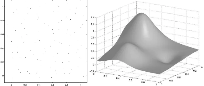
We consider here two tests, relating to the Franke (Test 1) and Nielson (Test 2) reference functions reported in Figure 1. Each displayed approximation is depicted together with the related data sample. For both considered tests a uniform 101×101 grid is used for the visualization and for the computation of the maximum (maxg) and root mean square (rmsg) errors. In all experiments below nmax = 2
Figure 1: Franke and Nielson parent surfaces on the left and on the right, respectively.
0 0.2 0.4 0.6 0.8 1 0
0.2 0.4 0.6 0.8 1
Figure 2: On the left the locations of the 100 data points for Test 1. On the rigth the related approximation.
In our first test, related to the Franke function, a small set of N =100 data points is used. It is available from [10] asds3and is shown on the left of Figure 2. The approximation depicted on the right of Figure 2 has been obtained using a uniform grid of size nx = ny = 5. The average number of knots used for the local hybrid
approximations is 23.9. The related grid errors are maxg = 1.5 ·10−2 and rmsg = 2.7 ·10−3. For comparison, using the same grid size the errors obtained with the original method and reported in [6] are maxg=3.8 ·10−2and rmsg=7.6 ·10−3(see Table 3 of that paper). In addition, we found in the literature the following errors for the interpolation of this data with the global multiquadric method: maxg=2.3 ·10−2 and rmsg=3.6 ·10−3in the famous Franke’s report [9], and rmsg=2.6 ·10−3in [3]. (In both cases a uniform 33×33 grid was used to compute the error.) Note that the above error from [3] corresponds to the case when a parameter value for multiquadric was found by optimization.
0 0.2 0.4 0.6 0.8 1 0
0.2 0.4 0.6 0.8 1
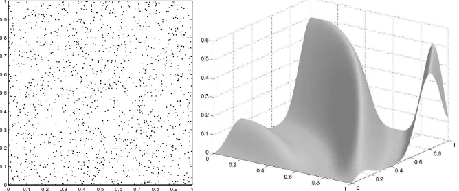
Figure 3: On the left the locations of the 200 data points for Test 2. On the rigth the related approximation.
0 0.1 0.2 0.3 0.4 0.5 0.6 0.7 0.8 0.9 1 0
0.1 0.2 0.3 0.4 0.5 0.6 0.7 0.8 0.9 1
set of 200 data points obtained evaluating this function on the locations corresponding to the data points available from [10] asds4. These locations are shown on the left of Figure 3. Again a uniform grid of size nx = ny = 5 is used. In this case the
approximation shown on the right of Figure 3 is obtained using an average knot number equal to 22 and the related grid errors are maxg=6.9 ·10−2and rmsg=1.4 ·10−2. For comparison, we mention that the same data set is used in [11] to test a least squares approximation method based on multiquadrics and parameter domain distortion. The best root mean square error (computed using a uniform 33×33 grid) reported in [11] is 1.3·10−2(see Table 1 and Figure 6 of that paper). Even if Figure 3 clearly shows some artifacts, we evaluate positively the results related to this first experiment for Test 2. In fact the accuracy and the shape recovery capability of our scheme are both comparable with those obtained in the best case reported in [11]. We would like also to say on this concern that, even if the results given in [11] have been obtained with remarkably few degrees of freedom, it should be taken into account that the parametric domain distortion method may encounter difficulties when applied to real data, as the authors admit [11, Section 4]. Finally, we get full shape recovery also for this challenging test function when we consider a denser set of 1500 scattered data depicted on the left of Figure 4 and use a finer spline grid by taking nx = ny = 8. The shape of the
corresponding approximation depicted on the right of Figure 4 is almost perfect now and the related grid errors are maxg=3.8 ·10−2and rmsg=1.3 ·10−3. The mean number of knots used in this case is 22.4.
References
[1] BOZZINIM.AND LENARDUZZIL., Bivariate knot selection procedure and
in-terpolation perturbed in scale and shape, to appear in: “Proceedings of the Fifth
Int. Conference on Curves and Surfaces”, Saint Malo 2002.
[2] BUHMANNM. D., Radial basis functions, Acta Numerica (2000), 1–38. [3] CARLSONR. E.ANDFOLEYT. A., Interpolation of track data with radial basis
methods, Comp. Math. with Appl. 24 (1992), 27–34.
[4] DAVYDOV O., On the approximation power of local least squares polynomials, in: “Algorithms for Approximation IV”, (Eds. Levesley J., Anderson I.J. and Mason J.C.) 2002, 346–353.
[5] DAVYDOV O.,MORANDI R.AND SESTINIA., Local hybrid approximation for
scattered data fitting with bivariate splines, preprint 2003.
[6] DAVYDOV O.ANDZEILFELDERF., Scattered data fitting by direct extension of
local polynomials to bivariate splines, Adv. Comp. Math., to appear.
[7] FARING., HOSCHEKJ. ANDKIM M. S., (Eds.), Handbook of computer aided
[8] FARING., Curves and surfaces for computer aided geometric design, Academic Press, San Diego 1993.
[9] FRANKER., A critical comparison of some methods for interpolation of scattered
data, Report NPS-53-79-003, Naval Postgraduate School 1979.
[10] FRANKE R., Homepage http://www.math.nps.navy.mil/∼rfranke/, Naval Postgraduate School.
[11] FRANKE R. AND HAGENH., Least squares surface approximation using
mul-tiquadrics and parametric domain distortion, Comput. Aided Geom. Design 16
(1999), 177–196.
[12] HABERJ., ZEILFELDERF., DAVYDOVO.ANDSEIDELH.-P., Smooth
Approx-imation and Rendering of Large Scattered Data Sets, in: “Proceedings of IEEE
Visualisation 2001” (Eds. Ertl T., Joy K. and Varshney A.), 2001 341–347, 571. [13] KANSAE. J. AND CARLSON R. E., Improved accuracy of multiquadric
inter-polation using variable shape parameters, Comp. Maths. with Appls. 24 (1992),
99–120.
[14] MORANDI R. AND SESTINIA., Geometric knot selection for radial scattered
data approximation, in: “Algorithms for Approximation IV”, (Eds. Levesley J.,
Anderson I.J. and Mason J.C.), 2002, 244–251.
[15] NIELSON G. M., A first order blending method for triangles based upon cubic
interpolation, Int. J. Numer. Meth. Engrg. 15 (1978), 308–318.
[16] STEWART G. W., Matrix Algorithms; Volume I: Basic Decompositions, SIAM, Philadelphia 1998.
AMS Subject Classification: 41A15, 65D10.
Oleg DAVYDOV Mathematisches Institut
Justus-Liebig-Universit¨at Giessen D-35392 Giessen, GERMANY
e-mail:[email protected]
Rossana MORANDI, Alessandra SESTINI Dipartimento di Energetica
Universit`a di Firenze, Via Lombroso 6/17 50134 Firenze, ITALY