Directory UMM :Journals:Journal_of_mathematics:OTHER:

(1)

DEL

S

EMINARIO

M

ATEMATICO

Universit`a e Politecnico di Torino

Splines, Radial Basis Functions and Applications

This special issue of Rendiconti del Seminario Matematico dell’Universit `a e del Politecnico di Torino contains the invited papers presented at the Workshop Giornate di studio su funzioni spline e funzioni radiali, held at the University of Torino, on February 5-7, 2003, in conclusion of the GNCS project Funzioni spline e funzioni ra-diali: applicazioni a problemi integrali e differenziali, Catterina Dagnino coordinator. The Workshop was supported by GNCS (Gruppo Nazionale per il Calcolo Scientifico).

As far as the program was concerned, there were three invited speakers: Armin Iske (Munich University of Technology, Germany), George Micula (Babes-Bolyai Uni-versity, Cluj-Napoca, Romania) and Paul Sablonni`ere (Institut National des Sciences Appliqu´ees, Rennes, France).

In addition, speakers from several Italian Universities provided papers for inclusion in the current issue, which were all refereed.

The contributions collected here deal with different aspects of numerical approx-imation based on splines and radial basis functions: a variational approach to spline functions theory, quadratic spline quasi-interpolants on bounded domains ofRd, d ₌ 1,2,3, basics and advanced topics on radial basis functions and meshfree methods for transport problems, a deficient spline collocation method for certain differential and integral equations with delay, some recent results on a new class of bivariate refinable functions, optimal nodal splines and their applications to integral problems, a local hybrid scheme for scattered data approximation, optimal center locations for radial ba-sis function interpolation, a collocation method for linear fourth order boundary value problems and closed spline curves bounding maximal area.

The invited papers appear according to their order during the oral presentation, the other ones in alphabetical order according to the author’s name.

The guest editors are deeply grateful to the authors who contributed to this issue. Moreover they thank Seminario Matematico, for taking care of the publication and GNCS for its support.

(3)

Splines and Radial Functions

G. Micula

∗

A VARIATIONAL APPROACH TO SPLINE FUNCTIONS

THEORY

Abstract. Spline functions have proved to be very useful in numerical analysis, in numerical treatment of differential, integral and partial dif-ferential equations, in statistics, and have found applications in science, engineering, economics, biology, medicine, etc. It is well known that in-terpolating polynomial splines can be derived as the solution of certain variational problems. This lecture presents a variational approach to spline interpolation. By considering quite general variational problems in ab-stract Hilbert spaces setting, we derive the concept of “abab-stract splines”. The aim of this leture is to present a sequence of theorems and results starting with Holladay’s classical results concerning the variational prop-erty of natural cubic splines and culminating in some general variational approach in abstract splines results. The whole exposition of this lecture is based on the papers of Champion, Lenard and Mills [24], [25].

1. Introduction

It is more than 50 years since I. J. Schoenberg ([56], 1946) introduced “spline func-tions” to the mathematical literature. Since then, splines, have proved to be enormously important in various brances of mathematics such as approximation theory, numerical analysis, numerical treatment of differential, integral and partial differential equations, and statistics. Also, they have become useful tools in field of applications, especially CAGD in manufacturing, in animation, in tomography, even in surgery.

Our aim is to draw attention to a variational approach to spline functions and to un-derline how a beautiful theory has evolved from a simple classical interpolation prob-lem. As we will show, the variational approach gives a new way of thinking about splines and opens up directions for theoretical developments and new applications.

Despite of so many results, this topics is not mentioned in many relevant texts on numerical analysis or approximation theory: even books on splines tend to mention the variational approach only tangentially or not at all.

Even though, there are recently published a few papers which underline the

vari-∗_{The author is very grateful to Professor Paul Sabloni`ere for helpful comments and additional references} during the preparation of fi nal form of this lecture. Extremly indebted is the author to Professors R. Cham-pion, C. T. Lenard and T. M. Mills for the kindness to send him the papers [24] and [25] on which basis this lecture has been preparated.

(4)

ational aspects of splines, and we mention the papers of Champion, Lenard and Mills ([25], 2000, [24], 1996) and of Beshaev and Vasilenko ([17], 1993).

The contain of this lecture is a completation of the excellent expository paper of Champion, Lenard and Mills [25]. We shall keep also the definitions and the notation from these papers.

The theorems and results of increasing generality or complexity which culminate in some general and elegant abstract results are not necessarily chronological.

2. Preliminaries

Notations:

R– the set of real numbers I : [a,b]_⊂R

P_m:_{= {}p_∈R_→R, p is real polynomial of degree _≤m, m_∈N_}

Hm(I):_{= {}x : I _→R, x(m−1)abs. cont. on I, x(m)_∈ L2(I), m_∈N, given_} If we define an inner product on Hm(I)by

(x1,x2):=

Z

I m

X

j=0

x₁(j)(t)x₂(j)(t)dt

then Hm(I)becomes a Hilbert space.

If X is a linear space, thenθXwill denote the zero element of X .

DEFINITION1. Let a ₌t0<t1 <· · ·<tn <tn+1 =b be a partition of I . The function s : I _→Ris a polynomial spline of degree m with respect to this partition if

• s_∈Cm−1(I)

• for each i _{∈ {}0,1, . . . ,n_}, s_|[ti,ti+j]∈Pm

The interior points_{t1,t2, . . . ,tn}are known as “knots”.

Natural cubic splines

Suppose that t1 < t2 < · · · < tn and{z1,z2, . . . ,zn} ⊂ Rare given. The classical

problem of interpolation is to find a “suitable” function8which interpolates the data point(ti,zi), 1≤i ≤n, that is:

8(ti)=zi, 1≤i ≤n.

(5)

THEOREM1 (HOLLADAY, 1957). If

• X :₌H2(I),

• a_≤t1<· · ·<tn≤b; n≥2,

• {z1,z2, . . . ,zn} ⊂R, and

• In:= {x∈ X : x(ti)=zi, 1≤i ≤n},

then_∃!σ _∈Insuch that

(1)

Z

I

[σ(2)(t)]2dt ₌min

Z

I

[x(2)(t)]2dt : x _∈ In

Furthermore,

• σ _∈C2(I),

• σ_|[ti,ti+1]∈P3for 1≤i≤n−1,

• σ_|[a,t1]∈P1andσ|[tn,b]∈P1.

From (1) we conclude thatσ is an optimal interpolating function – “optimal”, in

the sense that it minimize the functional

Z

I

[x(2)(t)]2dt over all functions in In. The

theorem goes on to state thatσ is a cubic spline function in the meaning of Schoenberg definition (1946). Asσ is linear outside [t1,tn] it is called “natural cubic spline”.

So, in a technical sense, we have found functions which are better than polynomials for solving the interpolation problem. Holladay’s theorem is most surprising not only because its proof is quite elementary, relying on nothing more complicated than inte-gration by parts, but it shows the intrinsec aspect of splines as solution of a variational problem (1) that has been a starting point to develop a variational approach to splines.

It is natural to ask: “Why would one choose to minimize

Z

I

[x(2)(t)]2dt?” For three reasons:

i) The curvature of functionσ isσ(2)/(1₊σ′2)3/2and so the natural cubic spline is the best in the sense that it approximates the interpolating function with mini-mum total curvature ifσ′is small.

(6)

iii) When presented with a set of data points(ti,zi), 1 ≤ i ≤ n, a statistician

can find a regression line which is the line of best fit in the least squares sense. This line is close to the data points Holladay’s theorem shows thatσ minimizes

Z

I

[x(2)(t)]2dt while still interpolating the data. We could say thatσ is an in-terpolating function which is “close to a straight lines” in that it minimizes this integral.

Thus, linear regression gives us

a straight line passing close to the points whereas Holladay’s result gives a curveσ which is

close to a straight line but passing through the points.

3. More splines

As we shall see, the Holladay’s theorem was the starting point in developing the varia-tional approach to splines. In what follows we shall describe a few of the many impor-tant generalizations and extensions of Holladay’s theorem.

Dm-splines

The next step was taken in 1963 by Carl de Boor [18] with the following result.

THEOREM2 (C.DEBOOR, 1963). If

• X :₌Hm(I),

• a_≤t1<t2<· · ·<tn ≤b; n ≥m,

• {z1,z2, . . . ,zn} ⊂Rand

• In:= {x∈ X : x(ti)=zi, 1≤i ≤n}

Z

I

[σ(m)(t)]2dt ₌min

Z

I

[x(m)(t)]2dt : x_∈ In

Furthermore,

• σ _∈C2m−2(I),

• σ_|[ti,ti+1]∈P2m−1, 1≤i ≤n−1, and

(7)

The function σ was called Dm-spline because it minimizes

Z

I

(Dmx)2dt, as x varies over In. The functionσ is called the interpolating natural spline function of

odd degree.

Clearly if we let m ₌2 in de Boor result, then we obtain Holladay result. For the even degree splines, such result was given by P. Blaga and G. Micula in 1993 [49], following the ideas of Laurent [44].

Trigonometric splines

In 1964, Schoenberg [57] changed the setting of the interpolation problem from the interval [a,b] to the unit circle: that is, from a non-periodic setting to a periodic setting. Similarly, let H₂k_π([0,2π ))denote the following space of 2π-periodic functions:

H₂k_π([0,2π )):_{= {}x : [0,2π )_→R: x₋2π₋periodic,

x(k−1)abs. cont. on [0,2π ), x(k)_∈L2₂_π([0,2π ))_}. THEOREM3 (SCHOENBERG, 1964). If

• X :₌H₂2m_π+1([0,2π ))

• 0_≤t1<t2<· · ·<tn<2π, n>2m+1

• {z1,z2, . . . ,zn} ⊂Rand

• T : X_→ L2₂_π([0,2π )), where T :₌D(D2₊12) . . . (D2₊m2),

Z 2π

0

[T(σ )(t)]2dt₌min

(Z 2π

0

[T(x)(t)]2dt : x _∈In

)

.

The optimal interpolating functionσis called the trigonometric spline. Schoenberg defined a trigonometric spline as a smooth function which in a particular piecewise trigonometric polynomial manner. He shows that trigonometric splines, so defined, provide the solution of this variational problem.

Note that the differential operator T has as K er T all the trigonometric polynomials of order m, that is, of the form:

x(t)₌a0+

m

X

j₌1

(8)

g-splines

Just over 200 years ago in 1870 Lagrange has constructed the polynomial of minimal degree such that the polynomial assumed prescribed values at given nodes and the derivatives of certain orders of the polynomial also assumed prescribed values at the nodes.

In 1968, Schoenberg [58] extended the idea of Hermite for splines. To specify that the orders of the derivatives specified may vary from node to node we introduce an incidence matrix E. As usual, let I :₌[a,b] be an interval partitioned by the nodes a _≤t1<t2<· · ·<tn ≤b. Let l be the maximum of the orders of the derivatives to

be specified at the nodes. The incidence matrix E is defined by:

E :₌(e(i,j): 1_≤i _≤n, 0_≤ j _≤l)₌:(e(i,j))

where each e(i,j)is 0 or 1. Assume also that each row of E and the last column of E contain a 1.

DEFINITION2. If m_≥1 is an integer, we will say that the incidence matrix E ₌ (e(i,j))is m-poised with respect to t1<t2<· · ·<tnif

• P _∈P_m₋₁_and

• e(i,j)₌1_⇒P(j)(ti)=0

together imply that P _≡0.

Now we can state Schoenberg’s result.

THEOREM4 (SCHOENBERG, 1968). If

• X :₌Hm(I)

• a_≤t1<t2<· · ·<tn ≤b

• E is an m-poised incidence matrix of dimension n_×(l₊1) • l<m_≤P_iP_je(i,j)

• {zi j : e(i,j)=1} ⊂Rand

• In:= {x∈ X : x(j)(ti)=zi jif e(i,j)=1}

Z

I

[σ(m)(t)]2dt₌min

Z

I

[x(m)(t)]2dt : x _∈ In

.

Schoenberg called the functionσ as g-spline from “generalized-splines”. Better may have been H-splines after Hermite or HB-splines after Hermite and Birkhoff.

(9)

L-splines

In 1967, Schultz and Varga [59] gave a major extension of the Dm-splines. Instead of the m-order derivative, operator Dm they considered a linear differential operator L creating a theory of so called L-splines. We shall state only one simple consequence of the many results of Schultz and Varga.

THEOREM5 (SCHULTZ ANDVARGA, 1967). If

• X :₌Hm(I)

• a_≤t1<t2<· · ·<tn ≤b; n ≥m

• {z1,z2, . . . ,zn} ⊂R

• In:= {x∈ X : x(ti)=zi, 1≤i ≤n}

• L : X _→ L2(I), so that L[x ](t) :₌

m

X

j=0

aj(t)Djx(t), where aj ∈ Cj(I),

0_≤ j_≤m, and_∃ω >0 such that am(t)≥ω >0 on I and

• L has P ´olya’s property W on I then_∃!σ _∈Insuch that

Z

I

[L[σ](t)]2dt₌min

Z

I

[L[x ](t)]2dt : x_∈ In

.

Clearly complexity is increasing with generality.

We note that L has P´olya’s property W on I if L[x ] ₌ 0 has m solutions x1,x2, . . . ,xmsuch that, for all t ∈ I and for all k∈ {1,2, . . . ,m}

det

   

x1(t) x2(t) . . . xm(t)

Dx1(t) Dx2(t) . . . Dxm(t)

. . . .

Dk−1x1(t) Dk−1x2(t) . . . Dk−1xm(t)

   6=0.

The relevance of P´olya’s property W is contained in the following sentence. To say that L has P´olya’s property W on I implies that, if L[x ]₌0 and x has m or more zeros on I , then x_≡0.

The optimal functionσ is known as an L-spline.

If L _≡ Dm we obtain the Dm-spline: so this is a major extension of previously stated results.

Schultz and Varga have defined an L-spline to be a smooth function constructed in a piecewise manner, where each piece is a solution of the differential equation L∗L x ₌0 where L∗is the formal adjoint of the operator L.

(10)

REMARK1. - The result of Schultz and Varga was proved in 1964 by Ahlberg, Nilson and Walsh [2]. They calledσ a “generalized splines”.

- The above result also follows from a paper of de Boor and Lynch [20] published in 1966.

- Perhaps the first paper along these lines of replacing the operator Dmby a more general differential operator was given by Greville [36] also in 1964. Unfortu-nately this often cited technical report was never published. Greville illustrates his method with an application to the classical numerical problem of interpo-lating mortality tables. Schultz and Varga applied their ideas to the numerical analysis of nonlinear two-point boundary value problems.

- Prenter [53] and Micula [50] are two of the few text books which touch this topic.

Lg-splines

Schoenberg extended the concept of Dm-splines to allow interpolation conditions of the Hermite type: this leads to g-splines. Schultz and Varga (and others) extended the concept of Dm-spline in a different direction by replacing the differential operator Dm by a more general operator: this leads to L-splines. The question is if one could combine both these extensions. In 1969 Jerome and Schumaker [31] combined these two extensions together in a very effective manner. One of their results is the following:

THEOREM6 (JEROME ANDSCHUMAKER, 1969). If

• X :₌Hm(I)

• {λ1, λ2, . . . , λn}is a set of linearly independent, continuous linear functionals

on X

• {z1,z2, . . . ,zn} ⊂R

• In:= {x∈ X : λi(x)=zi, 1≤i ≤n}

• L : X _→ L2(I)so that L[x ](t)₌

m

X

j=0

aj(t)Djx(t), aj ∈Cj(I), 0≤ j ≤ m,

and_∃ω >0 such that am(t)≥ω >0 on I and

• ker L_{∩ {}x _∈X : λi(x)=0, 1≤i ≤n} = {θX}

Z

I

[L[σ](t)]2dt₌min

Z

I

[L[x ](t)]2dt : x_∈ In

(11)

The optimal functionσis called the Lg-spline. The hypothesis about P´olya’s prop-erty W in Theorem 5 has with the more functional-analytic flavour. Jerome and Schu-maker allow interpolation conditions for the more general formλi(x)=zi, 1≤i ≤n,

whereλi (1 ≤ i ≤ n)are continuous linear functionals on X . This idea could cover

also others conditions like

Z ti+1

ti

x(t)dt ₌zi, 1≤i ≤n. We note also that they and

Laurent [44], pp. 225-226 replace the conditionsλi(x)=ziby z_i ≤λi(x)≤zi, where

z_iand zi (i =1,2, . . . ,n)are given real numbers with z_i ≤zi.

pLg-splines

For 1<p<_∞we define the space Hm(Ip)of functions by:

Hm,p(I):_{= {}x : I _→R: x(m−1)abs. cont., x(m)_∈ Lp(I)_} With a norm on Hm,p(I)defined by:

kx_km,p:= m

X

j=0

|x(j)(a)_{| +}

Z

I|

x(m)(t)_|pdt

1/p

the Hm,p(I)is a Hilbert space.

In 1978 Copley and Schumaker [26] established the following result:

THEOREM7 (COPLEY ANDSCHUMAKER, 1978). If

• X :₌Hm,p(I), p>1

• {λ1, λ2, . . . , λn}is a set of linearly independent continuous linear functionals on

X

• {z1,z2, . . . ,zn} ⊂R

• In:= {x∈ X : λi(x)=zi, 1≤i ≤n} 6= ∅

• L : X _→ Lp(I)so that L[x ](t)₌

m

X

j=0

aj(t)Djx(t), aj ∈Cj(I), 0≤ j ≤ m

and_∃ω >0 such that am(t)≥ω >0 on I , and

• ker L_{∩ {}x _∈X : λi(x)=0, 1≤i ≤n} = {θX}

then_∃!σ _∈Insuch that:

Z

I|

L[σ](t)_|pdt₌min

Z

I|

L[x ](t)_|pdt : x _∈ In

(12)

The optimal function σ is called a pLg-spline. For the first time, in this paper Copley and Schumaker have defined a pLg-spline to be a solution of the variational interpolation problem. One of the main problems that they investigated is to determine the structure of such splines. Can they be constructed in a piecewise manner? The com-plexity of their answer compensates the simplicity of their definition on a pLg-spline. In fact, Copley and Schumaker investigated more general interpolation problems. For example, they consider sets of linear functionals_{λα : α∈ A}where the index set A may be infinite, and also many extremly important examples.

Vector-valued Lg-splines

The following extension have come from researches in electrical engineering. In 1979 Sidhu and Weinert [60] consider the problem of simultaneous interpolation, that is, a method by which one could interpolate several functions at once.

THEOREM8 (SIDHU ANDWEINERT, 1979). If

• r_≥1, n1≥0, . . . ,nr ≥0 are fixed integers

• X :₌Hn1₍_I₎_×_Hn2₍_I₎_{× · · · ×}_Hnr₍_I₎

• {λ1, λ2, . . . , λn}is a set of linearly independent continuous linear functionals on

X

• {z1,z2, . . . ,zn} ⊂R

• In:= {x∈ X : λi(x)=zi, 1≤i ≤n}

• L : X _→L2(I)_{× · · · ×}L2(I)(an r -fold product), where

L[x ](t):₌

 

r

X

j₌1

Li j[xj](t): i =1,2, . . . ,r

  ′

,

Li j := nj

X

k₌0

ai j k(t)Dk; ai j nj =δi j; ai j k∈C

k₍_I_), ₀

≤k_≤nj, and

• ker L_{∩ {}x _∈X : λi(x)=0, 1≤i ≤n} = {θX}

then_∃!σ _∈X such that:

Z

I

(L[σ](t))′L[σ](t)dt₌min

Z

I

(L[x ](t))′L[x ](t)dt : x _∈ In

.

(Here A′indicates the transpose of the matrix or vector A.)

The optimal interpolating vector σ is known as a vector-valued Lg-spline. The authors have defined a vector-valued Lg-spline to be the solution of a variational in-terpolation problem, proved the existence-uniqueness theorem and then discussed an algorithm for calculating such splines in the special case that the functionalλi are of

(13)

Thin plate splines

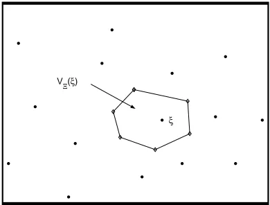
So far we have been considering the problem of interpolating functions of a single variable. In 1976, Jean Duchon [29], [23] - [27] - [28] developed a variational approach to interpolating functions of several variables. We will state his result only for functions of two variables. We denote an arbitrary element ofR2_{by t}₌_(ξ

1, ξ2),ktk2:=ξ₁2+ξ₂2 and the set of linear polynomials by:

P₁:_{= {}p1(t)=a0+a1ξ1+a2ξ2: {a0,a1,a2} ⊂R}. THEOREM9 (DUCHON, 1976). If

• X :₌H2(R2),

• {t1,t2, . . . ,tn} ⊂R2such that if p1∈ P1and p1(t1)= · · · = p1(tn)=0, then

p1≡0,

• {z1,z2, . . . ,zn} ⊂R,

• In:= {x∈ X : x(ti)=zi, 1≤i ≤n}and

• J : X_→Rsuch that

J(x):₌

Z Z

R2 

 ∂2x

∂ξ₁2

!

+2 ∂ 2_x

∂ξ1∂ξ2

!2

+ ∂

2_x

∂ξ₂2

! dξ1dξ2

J(σ )₌min_{J(x): x_∈ In}.

Furthermore,_∀t_∈R2

σ (t)₌

n

X

j=1

µikt−tik2lnkt−tik +p1(t)

where p1∈P1and(∀q ∈P1),

n

X

i₌1

µiq(ti)=0

!

.

The optimal functionσ is known as a “thin plate spline”. The dramatic aspect of this result is the form of the splineσ: it is no a piecewise polynomial function.

This two-dimensional result appeared almost 20 years after Holladay’s one-dimensional result. The delay is not so surprising. Holladay’s proof involves noth-ing more complicated than integration by parts whereas Duchon’s paper uses tempered distribution, Radon measure and other tools from functional analysis.

(14)

ii) Duchon was not the first person to investigate the multivariate problem. In 1972 the work of two aircraft engineers Harder and Desmarais [37] approached this problem from an applied point of view. In 1974 Fisher and Jerome [32] ad-dressed the multivariate problem. In 1970, J. Thomann [62] in his doctoral thesis considered a variational approach to interpolation on a rectangle or on a disk in R2. The book by Ahlberg, Nilson and Walsh [3] also deals with multivariate problems, but from a point of view which is essentially univariate.

Yet more splines

The overture of splines could be continued. There are other many splines associated with some variational interpolation problems and for each case we could state a theo-rem similar to those above. We shall only nominate they:

3-splines (1972, Jerome and Pierce [41]) LMg-splines (1979, R. J. P. de Figueiredo [30]) ARMA-splines (1979, Weinert, Sesai and Sidhu [67]) Spherical splines (1981, Freeden, Scheiner and Franke [33]) PDLg-splines (1990, R. J. P. de Figueiredo and Chen [31]) Polyharmonic splines (1990, C. Rabut [54])

Vector splines (1991, Amodei and Benbourhim [5])

Hyperspherical splines (1994, Taijeron, Gibson and Chandler [61]).

4. Abstract splines

The statements of the above theorems were becoming quite long and complicated. But, there is a general abstract result which captures the essence of most of them. The following result is attributed to M. Atteia [10], [11],[12] - [15], and it relates to following diagram:

X

A

T //_Y

Z THEOREM10 (ATTEIA, 1992). If

• X,Y,Z are Hilbert spaces,

• T,A are continuous linear surjections,

• z_∈ Z

• ker T ₊ker A is closed in X ,

(15)

• I(z)_{= {}x_∈ X : Ax₌z_} then_∃!σ _∈I(z)such that:

kTσ_kY =min{kT xkY : x∈ I(z)}.

The optimalσ is known as a variational interpolating spline.

To illustrate that this theorem reflects the essence of the most above results, let us see how it generalizes Theorem 1 of Holladay. Put X ₌H2(I), Y ₌L2(I), Z ₌Rn, T x :₌ x(2), Ax :₌(x(t1),x(t2), . . . ,x(tn)). All the hypotheses of Atteia’s theorem

are satisfied. Atteia’s theorem does not cover all the above results, e.g. Theorem 7 which deals with pLg-splines.

- An equivalent result to Atteia’s theorem is found in the often cited, but unfortu-nately never published, report by Golomb [34] in 1967.

- The essential ideas also can be found in Anselone and Laurent [6] in 1968 and in the classic book by Laurent [44], entitled Approximation et Optimisation (Her-man, Paris, 1972).

There are important remarks to be made about this theorem.

1. The role of the condition about ker T ₊ker A is to ensure the existence ofσ whereas the role of the condition ker T_∩ker A is to ensure the uniqueness ofσ. This separation was made clear by Jerome and Schumaker [42] in 1969.

2. The challenge of any abstract theory is to generalize a wide variety of particular cases, and simultaneously, preserve as much of the detail as possible. To a large extent, Atteia and others have, over many years, being doing this in the case that X is a reproducing kernel Hilbert space. Details of this theory can be found in the excellent monographs of Atteia ([11], 1992) and Bezhaev and Vasilenko ([17], 1993). The origins of this program can be found in 1959 paper by Golomb and Weinberger [35], in Habilitation Thesis of Atteia ([10], 1966) and in 1966 paper by de Boor and Lynch [20].

3. The above general theorem can itself be generalized in many directions.

One generalization enables us to consider constrained interpolation problems which are very important in contemporary mathematics. It is due to Atteia [10] and Utreras, [63] in 1987 and relates to the following diagram

C_⊂X

A

T _/_/

Y

(16)

THEOREM11 (UTRERAS, 1987). If

• X,Y,Z are Hilbert spaces,

• C is a closed, convex subset of X ,

• z_∈ Z

• A,T are continuous, linear surjections,

• w_∈I(C,z):_{= {}x_∈C : Ax ₌z_}

• ker T ₊(ker A_∩(C₋w))is closed in X and

• ker A_∩ker T _{= {}θX}

then_∃!σ _∈I(C,z)such that

kTσ_kY =min{kT xkY : x ∈ I(C,z)}.

If we put C ₌X then we obtain Theorem 10 of Atteia. Utreras’ theorem is useful if, for example, we want to interpolate positive data by positive functions. In this case we have X₌Hm(I)and C is the set of positive function in X .

Other generalizations have extended Atteia’s theorem to Banach spaces settings, rather than Hilbert spaces. So that are known the following new splines in Banach spaces:

R-splines (1972, Holmes [40])

M-splines (1972, Lucas [47], 1985 Abraham [1]) Lf-splines (1983, Pai [51])

Tf-splines (1993, Benbourhim and Gaches [16]).

A key work in the Banach space setting is the 1975 paper of Fischer and Jerome [32], where the perfect splines are very important in this contex.

5. Conclusions and comments

The book of Laurent ([44], 1972) was perhaps the first book which emphasized the variational approach to splines.

Atteia’s book ([11], 1992) is the key work in this area, especially for those inter-ested in functional analysis.

Whaba ([66], 1990) is the first book describing applications of these ideas (in smoothing rather the interpolation) to statistics.

Bezhaev and Vasilenko ([17], 1993) published in Novosibirsk entitled “Variational Spline Theory” contains the most abstracts and rigorous results in this field.

(17)

1. Splines may be defined as solution of variational problems rather than functions constructed in some piecewise manner. We have seen that these variational prob-lems have become increasingly abstract and hence the concept of “splines” has became increasingly abstract. This may not be everyone’s liking, at least, ini-tially. For example, in 1966 in [20] de Boor and Lynch have written: “in order not to dilute the notion of spline functions too much, we prefer to follow Gre-ville’s definition of a general spline function” – which is based on a piecewise, constructive approach. In any case, the variational theory gives us a new appre-ciation of the concept of a “spline”.

2. The variational approach facilitates a natural, attractive way to extend the clas-sical theory of interpolating splines, especially to multivariate situations. The works of Duchon [29], [23] - [27] - [28], in 1976 and Whaba [65] in 1981 illus-trate this conclusion. More recently, in 1993, de Boor [19] changing his earlier opinion wrote: “I am convinced that the variational approach to splines will play a much greater role in multivariate spline theory that it did or should have in univariate theory”.

3. The theory of variational splines demonstrates the power of functional analysis to yield a unified approach to computational problems in interpolation. As S. Sobolev [45], one year before his dead has been quoted: “It is impossible to image the theory of computations with no Banach spaces”.

References

[1] ABRAHAMA., On the existence and uniqueness of M-splines, J. Approx. Theory 43 (1985), 36–42.

[2] AHLBERG J.H., NILSON E.N. AND WALSH J.L., Fundamental properties of generalized splines, Proc. Nat. Acad. Sci. USA 52 (1964), 1412–1419.

[3] AHLBERGJ.H., NILSONE.N.ANDWALSHJ.L., The theory of splines and their applications, Academic Press, New York 1967.

[4] AMODEI L., Étude d’une classe de fonctions splines vectorielles en vue de l’approximation d’un champ de vitesse. Applications à la météorologie, Thèse, Université Paul Sabatier, Toulouse 1993.

[5] AMODEI L. AND BENBOURHIM M.N., A vector spline approximation, J. Ap-prox. Theory 67 (1991), 51–79.

[6] ANSELONEP.M.ANDLAURENTP.J., A general method for the construction of interpolating or smoothing spline-functions, Numer. Math. 12 (1968), 66–82. [7] APPRATOD., ARCANGELI R.ANDGACHESJ., Fonctions spline par moyennes

(18)

[8] APPRATOD., ARCANGELI R.ANDGACHESJ., Fonctions spline par moyennes locales sur un ouvert borne de I Rn, Ann. Facul. des Sci. Toulouse V (1983), 61–87.

[9] ATTEIAM., Généralisation de la définition et des propriétés des spline fonctions, C. R. Acad. Sc. Paris 260 (1965), 3550–3553.

[10] ATTEIAM., Étude de certains noyaux et théorie des fonctions spline en analyse numérique, Thèse d’Etat, Instit. Math. Appl., Grenoble 1966.

[11] ATTEIAM., Hilbertian kernels and spline functions, North Holland, Amsterdam 1992.

[12] ATTEIAM., Fonctions splines généralisées, Sci. Paris 261 (1965), 2149–2152.

[13] ATTEIAM., Existence et d´etermination des fonction - spline `a plusieurs vari-ables, C.R. Acad. Sci. Paris, 262 (1966), 575–578.

[14] ATTEIAM., Fonctions - splines et noyaux reproduisants d’ Aronszajn - Bergman, Re. Franc. d’Inf. et de Rech. Oper. R3 (1970), 31–43.

[15] ATTEIAM., Fonctions - splines definies dans un ensemble convexe, Num. Math. 12 (1968), 192–210.

[16] BENBOURHIM N.M. AND GACHES J., Tf-splines et approximation par Tf

-prolongement, Studia Math. 106 (1993), 203–211.

[17] BEZHAEVA.YU.ANDVASILENKOV.A., Variational spline heory, Novosibirsk Computing Center, Novosibirsk 1993.

[18] DEBOORC., Best approximation properties of spline functions of odd degree, J. Math. Mech. 12 (1963), 747–749.

[19] DE BOORC., Multivariate piecewise polynomials, Acta Numerica (1993), 65– 109.

[20] DE BOOR C. AND LYNCH R.E., On spline and their minimum properties, J. Math. Mech. 15 (1966), 953–969.

[21] BOUHAMIDIA., Interpolation et approximation par des fonctions splines radi-ales `a plusieurs variables, Th`ese, Univ. de Nantes, Nantes 1992.

[22] BOUHAMIDIA.ANDLEM ÉHAUTE´A., Splines curves et surfaces under tension, in: “Wavelets, Image and Surface Fitting” (Eds. Laurent P.J., Le Méhauté A., Schumaker L.L. and Peters A.K.), Wellesley 1994, 51–58.

[23] BOUHAMIDI A. AND LE M ´EHAUTE´ A., Hilbertian approach for univariate spline with tension, ATA 17 4 (2001), 36–57.

(19)

[25] CHAMPIN R., LENARD C.T. AND MILLS T.M., A variational approach to splines, The ANZIAM J. 42 (2000), 119–135.

[26] COPLEY P. AND SCHUMAKER L.L., On p Lg-splines, J. Approx. Theory 23 (1978), 1–28.

[27] DUCHON J., Splines minimizing rotation-invariant semi-norms in Sobolev spaces, LNM 571, Springer Verlag 1977, 85–100.

[28] DUCHONJ., Sur l’erreur d’interpolation des fonctions de plusieurs variables par Dm- splines, RAIRO Anal. Numer. 12 4 (1978), 325–334.

[29] DUCHONJ., Interpolation des fonctions de deux variables suivant le principle de la flexion des plaques minces, R.A.I.R.O. Analyse Num´erique 10 (1976), 5–12. [30] DEFIGUEIREDOR.J.P., Lm-g-splines, J. Approx. Theory 19 (1979), 332–360.

[31] DE FIGUEIREDO R.J.P. AND CHEN G., P D Lg splines defined by partial

dif-ferential operators with initial and boundary value condiitons, SIAM J. Numer. Anal. 27 (1990), 519–528.

[32] FISHER S.D. AND JEROME J.W., Elliptic variational problems in L2 in L∞, Indiana Univ. Math. J. 23 (1974), 685–698.

[33] FREEDEN W., SCHREINERM. AND FRANKE R., A survey of spherical spline approximation, Surveys on Mathematics for Industry, 1992.

[34] GOLOMB M., Splines, n-widths and optimal approximations, MRC Technical Summary Report 784, Mathematics Research Center, US Army, Wisconsin 1967.

[35] GOLOMB M. AND WEINBERGER H.F., Optimal approximation and error bounds, in: “On Numerical Approximation” (Ed. Langer R.E.), Univ. Wiscon-sin Press, Madison 1959, 117–190.

[36] GREVILLE T.N.E., Interpolation by generalized spline functions, MRC Tech-nical Summary Report 476, Mathematics Research Center, US Army, Madison, Wisconsin 1964.

[37] HARDER R.L. AND DESMARAIS R.N., Interpolation using surface splines, J. Aircraft 9 (1972), 189–191.

[38] HOLLADAYJ.C., A smoothest curve approximation, Math. Tables Aids Comput. 11 (1957), 233–243.

[39] HOLLANDA.S.B.AND SAHNEYB.N., The general problem of approximation and spline functions, Robert E. Krieger Publ., Huntington 1979.

(20)

[41] JEROMEJ.W.AND PIERCEJ., On spline functions determined by singular self-adjoint differential operators, J. Approx. Theory 5 (1972), 15–40.

[42] JEROME J.W. AND SCHUMAKER L.L., On Lg-splines, J. Approx. Theory 2 (1969), 29–49.

[43] JEROMEJ.W.ANDVARGAR.S., Generalizations of spline functions and appli-cations to nonlinear boundary value and eigenvalue problems, in: “Theory and Applications of Spline Functions” (Ed. Greville T.N.E.), Academic Press, New York 1969, 103–155.

[44] LAURENTP.J., Approximation et optimisation, Hermann, Paris 1972.

[45] LEBEDEVV.I., An introduction to functional analysis and computational mathe-matics, Birkh¨auser, Boston 1997.

[46] LUCAS T.R., A theory of generalized splines with applications to nonlinear boundary value problems, Ph. D. Thesis, Georgia Institute of Technology 1970. [47] LUCAST.R., M-splines, J. Approx. Theory 5 (1972), 1–14.

[48] MICULAG., Funct¸ii spline s¸i aplicat¸ii, Tehnic˘a, Bucures¸ti 1978.

[49] MICULAG.ANDBLAGAP., Natural spline function of even degree, Studia Univ. Babes¸-Bolyai Cluj-Napoca, Series Mathematica 38 (1993), 31–40.

[50] MICULAG.ANDMICULAS., Handbook of Splines, Kluwer Academic Publish-ers, Dordrecht-Boston-London 1999.

[51] PAID.V., On nonlinear minimization problems and Lf-splines. I, J. Approx. The-ory 39 (1983), 228–235.

[52] POWELLM.J.D., The theory of radial basis function approximation, Adv. Num. Anal. Vol.II (Ed. Light W.), OUP, Oxford 1992.

[53] PRENTER P.M., Splines and variational methods, John Wiley and Sons, New York 1975.

[54] RABUTC., B-splines polyharmoniques cardinales: interpolation, quasi-interpo-lation, filtrage, Th`ese, Universit´e Paul Sabatier, Toulouse 1990.

[55] SCHABACK R., Konstruktion und algebraische Eigenschaften von M-Spline-Interpolierenden, Numer. Math. 21 (1973), 166–180.

[56] SCHOENBERGI.J., Contribution to the problem of approximation of equidistant data by analytic functions, Parts A and B, Quart. Appl. Math. 4 (1946), 45–99, 112–141.

(21)

[58] SCHOENBERGI.J., On the Ahlberg-Nilson extension of spline interpolation: The g-splines and their optimal properties, J. Math. Anal. Appl. 21 (1968), 207–231. [59] SCHULTZM.H.ANDVARGAR.S., L-splines, Numer. Math. 10 (1967), 345–369.

[60] SIDHU G.S. AND WEINERT H.L., Vector-valued Lg-splines. I. Interpolating splines, J. Math. Anal. Appl. 70 (1979), 505–529.

[61] TAIJERON H.J., GIBSON A.G. AND CHANDLER C., Spline interpolation and smoothing on hyperspheres, SIAM J. Sci. Comput. 15 (1994), 1111–1125. [62] THOMANNJ., D´etermination et construction de fonctions spline `a deux variables

définies sur un domaine rectangulaire ou circulaire, Thèse, Université de Lille, Lille 1970.

[63] UTRERAS F.I., Convergence rates for constrained spline functions, Rev. Mat. Appl. 9 (1987), 87–95.

[64] VARGA R.S., Functional analysis and approximation theory, SIAM, Philadel-phia 1971.

[65] WAHBAG., Spline interpolation and smoothing on the sphere, SIAM J. Sci. Stat. Comp. 2 (1981), 5–16.

[66] WAHBAG., Spline models for observational data, SIAM, Philadelphia 1990.

[67] WEINERT H.L., SESAIU.B. ANDSIDHUG.S., Arma splines, system inverses, and least-squares estimates, SIAM J. Control Optim. 17 (1979), 525–536.

AMS Subject Classification: 65D07, 41A65, 65D02, 41A02.

Gheorghe MICULA Babes¸-Bolyai University

Department of Applied Mathematics 3400 Cluj-Napoca, ROMANIA

(22)

(23)

Splines and Radial Functions

P. Sablonni`ere

∗

QUADRATIC SPLINE QUASI-INTERPOLANTS ON BOUNDED

DOMAINS OF

_R

d, d

₌

1 ,

2 ,

3

Abstract. We study some C1 quadratic spline quasi-interpolants on bounded domains_⊂Rd,d ₌1,2,3. These operators are of the form Q f(x) ₌ P_k_∈_K₍₎µk(f)Bk(x), where K()is the set of indices of

B-splines Bk whose support is included in the domainand µk(f)is

a discrete linear functional based on values of f in a neighbourhood of xk ∈ supp(Bk). The data points xj are vertices of a uniform or

nonuni-form partition of the domainwhere the function f is to be approximated. Beyond the simplicity of their evaluation, these operators are uniformly bounded independently of the given partition and they provide the best ap-proximation order to smooth functions. We also give some applications to various fields in numerical approximation.

1. Introduction and notations

In this paper, we continue the study of some C1quadratic (or d-quadratic) spline dis-crete quasi-interpolant(dQIs) on bounded domains _⊂ Rd,d ₌ 1,2,3 initiated in [36]. These operators are of the form Q f(x)₌ P_k_∈_K₍₎µk(f)Bk(x), where K()

is the set of indices of B-splines Bk whose support is included in the domainand

µk(f)is adiscrete linear functionalP_i_∈_I₍_r₎λk(i)f(xi₊k), with I(r)=Zd∩[−r,r ]d

for r _∈N_{fixed (and small). The data points x}_j _{are vertices of a uniform or nonuniform} partition of the domainwhere the function f is to be approximated. Such operators have been widely studied in recent years (see e.g. [4], [6]-[11],[14], [23], [24], [31], [38], [40] ), but in general, except in the univariate or multivariate tensor-product cases, they are defined on thewhole spaceRd: here we restrict our study tobounded domains and to C1quadratic splinedQIs. Their main interest lies in the fact that they provide approximants having the best approximation order and small norms while being easy to compute. They are particularly useful as initial approximants at the first step of a multiresolution analysis. First, we study univariate dQIs on uniform and non-uniform meshes of a bounded interval of the real line (Section 2) or on bounded rectangles of the plane with a uniform or non-uniform criss-cross triangulation (Section 3). We use

∗_{The author thanks very much prof.} _{Catterina Dagnino, from the Dipartimento di Matematica} dell’Universit`a di Torino, and the members of the italian project GNCS on spline and radial functions, for their kind invitation to theGiornate di Studio su funzioni spline e funzioni radiali, held in Torino in February 6-7, 2003, where this paper was presented by the author.

(24)

quadratic B-splines whose Bernstein-B´ezier (abbr. BB)-coefficients are given in tech-nical reports [37], [38] and which extend previous results given in [12]. In the same way, in section 4, we complete the study of a bivariate blending sum of two univariate dQIs of Section 1 on a rectangular domain. Finally, in Section 5, we do the same for a trivariate blending sum of a univariate dQI (Section 1) and of the bivariate dQI de-scribed in Section 2. For blending and tensor product operators, see e.g. [2], [3], [16], [18], [19], [20], [21], [30]. For some of these operators, we improve the estimations of infinite norms which arebounded independently of the given partitionof the domain. Using the fact that the dQI S is exact on the spaceP₂ _∈ S₂of quadratic polynomials and a classical result of approximation theory:_kf₋S f_{k ≤}(1_+kS_k)d(f,S₂)(see e.g. [15], chapter 5), we conclude that f ₋S f ₌O(h3)for f smooth enough, where h is the maximum of diameters of the elements (segments, triangles, rectangles, prisms) of the partition of the domain. But we specify upper bounds for some constants occuring in inequalities giving error estimates for functions and their partial derivatives of total order at most 2. Finally, in Section 6, we present some applications of the preced-ing dQIs, for example to the computation of multivariate integrals, to the approximate determination of zeros of functions, to spectral-type methods and to the solution of integral equations. They are still in progress and will be published elsewhere.

2. Quadratic spline dQIs on a bounded interval

Let X _{= {}x0,x1, . . . ,xn}be a partition of a bounded interval I =[a,b] , with x0=a and xn =b. For 1 ≤i ≤n, let hi = xi−xi−1be the length of the subinterval Ii =

[xi−1,xi]. LetS2(X)be the n+2-dimensional space of C1quadratic splines on this partition. A basis of this space is formed by quadratic B-splines_{Bi,0≤i ≤ n+1}.

Define the set of evaluation points

2n= {θ0=x0, θi =

1

2(xi−1+xi), f or 1≤i ≤n, θn+1=xn}.

The simplest dQI associated with 2n is the Schoenberg-Marsdenoperator (see e.g.

[25], [36]):

S1f :=

n₊1

X

i=0 f(θi)Bi

This operator is exact onP₁. Moreover S1e2=e2+Pni=114h 2

iBi. We have studied in

[1] and [36] the unique dQI of type

S2f = f(x0)B0+

n

X

i₌1

µi(f)Bi+ f(xn)Bn+1

whose coefficient functionals are of the form

(25)

and which is exact on the spaceP₂ _{of quadratic polynomials. Using the following} notations and the convention h0=hn₊1=0, we finally obtain, for 1≤i ≤n:

σi =

hi

hi−1+hi

, σ_i′₌ hi−1

hi−1+hi =

1₋σi,

ai = −

σ_i2σ_i′₊₁

σi+σ_i′₊₁

, bi =1+σiσi′₊1, ci = −

σi(σ_i′₊₁)2

σi+σ_i′₊₁

.

Defining the fundamental functions of S2by

˜

B0=B0+a1B1,

˜

Bi =ci−1Bi−1+biBi+ai+1Bi+1, 1≤i ≤n,

˜

Bn+1=cnBn+Bn+1, we can express S2f in the following form

S2f =

n+1

X

i₌0

f(θi)B˜i.

In [26] (see also [22] and [32], chapter 3), Marsden proved the existence of a unique Lagrange interpolantL f inS₂₍_X₎_{satisfying L f}_(θ_i₎₌ _f_(θ_i₎_{for 0} _≤_i _≤_n₊_{1. He} also proved the following

THEOREM 1. For f bounded on I and for any partition X of I , the Chebyshev norm of the Lagrange operator L is uniformly bounded by 2.

Now, we will prove a similar result for the dQI S2defined above. It is well known that the infinite norm of S2is equal to the Chebyshev norm of the Lebesgue function

32=Pin₌+01| ˜Bi|of S2.

THEOREM2. For f bounded on I and for any partition X of I , the infinite norm of the dQI S2is uniformly bounded by 2.5.

Proof. Each function_{| ˜}Bi| being bounded above by the continuous quadratic spline

¯

Bi whose BB-coefficients are absolute values of those of B˜i, we obtain 32 ≤

¯

32 = Pn_i₌+₀1B¯i. So, we have to find an upper bound of 3¯2. First, we need the BB-coefficients of the fundamental functions: they are computed as linear combi-nations of the BB-coefficients of B-splines. In order to avoid complicated nota-tions, we denote by [a,b,c] the triplet of BB-coefficients of the quadratic polynomial a(1₋u)2₊2bu(1₋u)₊cu2_{for u} _∈ _[0_,_{1]. Any function g} _∈ _S

2(X)can be writ-ten in this form on each interval [xi−1,xi],1 ≤ i ≤ n, with the change of variable

u ₌(x₋xi−1)/hi. So, the BB-coefficients of g consist of a list of n triplets. Let us

denote by L(i)the list associated with the functionB˜i (we do not write the triplets of

null BB-coefficients). Setting, for 1_≤i _≤n₋1:

(26)

we obtain for the three first functionsB˜0,B˜1,B˜2:

L(0)₌[1,a1,a1σ2],[a1σ2,0,0] L(1)₌[0,b1,e1],[e1,a2,a2σ3],[a2σ3,0,0] L(2)₌[0,c1,d1],[d1,b2,e2],[e2,a3,a3σ4],[a3σ4,0,0] For 3_≤i _≤n₋2 (general case), we have supp(B˜i)=[xi₋3,xi₊2] and L(i)₌[0,0,ci₋1σi′₋1],[ci₋1σi′₋1,ci₋1,di₋1],[di₋1,bi,ei],

[ei,ai+1,ai+1σi+2],[ai+1σi+2,0,0] Finally, for the three last functionsBñ₋1,Bñ,Bñ₊1, we get:

L(n₋1)₌[0,0,cn−2σn′−2],[cn−2σn′−2,cn−2,dn−2],[dn−2,bn−1,en−1],[en−1,an,0]

L(n)₌[0,0,cn−1σn′−1],[cn−1σn′−1,cn−1,dn−1],[dn−1,bn,0]

L(n₊1)₌[0,0,cnσn′],[cnσn′,cn,1]

We see that di ≥0 (resp. ei ≥0), for it is a convex combination of ci and bi₊1(resp. of bi and ai₊1), with bi ≥ 1 and|ci|and|ai| ≤ 1 for all i . Therefore, the absolute

values of the above BB-coefficients (i.e. the BB-coefficients of the B¯_i′s) are easy to evaluate. Now, it is easy to compute the BB-coefficients of the continuous quadratic spline3¯2=Pni₌+01B¯i. On each interval [xi−1,xi], for 2≤i ≤n−1, we obtain

[λi₋1, µi, λi]=[−ai₋1σi+di₋1+ei₋1−ciσi′,bi−ai−ci,−aiσi₊1+di+ei−ci₊1σi′₊1] For the first (resp. the last) interval, we haveλ0 =1 (resp. λn =1) For the central

BB-coefficient, we get, sinceσi andσ_i′are in [0,1] for all indices:

µi =bi −(ai+ci)=2bi−1=1+2σiσi′+1≤3 For the extreme BB-coefficients, we have, since ai+bi+ci =1:

λi =(1−2ai)σi₊1+(1−2ci₊1)σi′₊1=1+

2(σi)2σi₊1σ_i′₊₁

σi+σ_i′₊₁ +

2σi₊1σ_i′₊₁(σ_i′₊₂)2

σi+1+σ_i′₊₂

.

Let us consider the rational function f defined byλi =1+ f(σi, σi+1, σi+2):

f(x,y,z)₌ 2x

2_y₍₁

−y) 1₊x₋y +

2y(1₋y)(1₋z)2 1₊y₋z ,

the three variables x,y,z lying in the unit cube. Its maximum is attained at the vertices

{(0,1,0), (1,0,0), (1,0,1), (1,1,0)_}and it is equal to 1. This proves thatλi ≤ 2

for all i . Therefore, in each subinterval (after the canonical change of variable),3¯2is bounded above by the parabola:

(27)

Now, we consider the case of auniform partition, say with integer nodes for

sim-It is easy to see that, in order to compute_kS2k_∞, it suffices to evaluate the maximum of the Lebesgue function on the subinterval J ₌[0,4]. Here are the lists L(i)of the BB-coefficients of the fundamental functions_{{ ˜}Bi,0 ≤ i ≤ 6}whose supports have

at least a common subinterval with J . As in the nonuniform case, we only give the triplets associated with subintervals of supp(B˜i)∩J :

supp(B˜0)∩J =[0,2], L(0)=

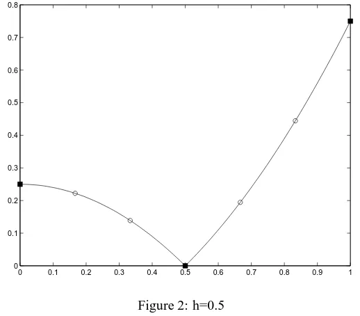
Drawing32reveals that the abscissax of its maximum lies in the interval [0¯ .6,1]. In this interval, we obtain successively:

(28)

whence3′₂(x)₌ ₁₂1(64₋69x)andx_¯₌ 64₆₉. This leads to

kS2k∞= k32k∞=32(x¯)= 305

207≈1.4734.

So, we have proved the following result:

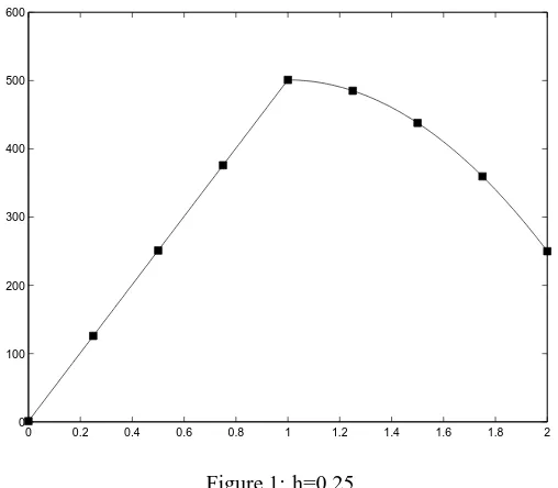
THEOREM 3. For uniform partitions of the interval I , the infinite norm of S2is equal to305₂₀₇ _≈1.4734.

REMARK1. Further results on various types of dQIs will be given in [21].

Now, we will give somebounds for the error f ₋S2f . Using the fact that the dQI S2is exact on the subspaceP2 ⊂ S2of quadratic polynomials and a classical result of approximation theory (see e.g. [17], chapter 5), we have for all partitions X of I in virtue of Theorem 4:

kf ₋S2fk∞≤(1+ kS2k∞)di st(f,S2)∞≤3.5 di st(f,S2)∞

So, the approximation order is that of the best quadratic spline approximation. For example, from [17], we know that for any continuous function f

di st(f,S₂)_∞_≤3ω(f,h)_∞ where h₌max_{hi,1≤i ≤n}, so we obtain

kf ₋S2fk_∞≤10.5ω(f,h)_∞

But a direct study allows to decrease the constant in the right-hand side.

THEOREM4. For a continuous function f , there holds:

kf ₋S2fk∞≤6ω(f,h)∞

Proof. For any x_∈ I , we have

f(x)₋S2f(x)=

n₊1

X

i=0

[ f(x)₋ f(θi)]B˜i(x)

Assuming n_≥5 and x _∈ Ip=[xp−1,xp], for some 3≤ p≤n−2, this error can be

written, since supp(B˜i)=[xi−3,xi+2]:

f(x)₋S2f(x)=

p₊2

X

i=p−2

(29)

Asθi = 1₂(xi₋1+xi), we have|x−θi| ≤rih, with ri = |p−i| +0.5. Using a well

so, we obtain finally a lower constant (but not the best one) in the right-hand side of the previous inequality:

kf ₋S2fk∞≤6ω(f,h)∞

Now, let us assume that f _∈C3(I), then we have the following

THEOREM5. For all function f _∈C3(I)and for all partitions X of I , the follow-ing error estimate holds, with C0≤1:

kf ₋S2fk_∞≤C0h3kf(3)k_∞ which can be written explicitly as

(30)

As_|Rθi

x (θi−s)2ds| ≤

1

3|x−θi|3, we get the following upper bound:

|S2f(x)− f(x)| ≤ 1 6kf

(3)

k∞

p+2

X

i₌p₋2

|x₋θi|3B¯i(x)

≤ h

3

6 kf (3)

k∞

p₊2

X

i=p−2

(_|p₋i_{| +}1 2)

3_B_¯

i(x)

As in the proof of theorem above, and without going into details, one can prove that the last sum in the r.h.s. is uniformly bounded by 6 for any partition of I . So, we obtain finally:

|S2f(x)− f(x)| ≤h3kf(3)k_∞

By using the same techniques, the results of theorem 5 can be improved when X is auniform partitionof I :

THEOREM6. (i) For f _∈C(I), there holds:

|S2f(x)− f(x)| ≤2.75ω(f, h 2)∞

(ii) for f _∈C3(I)and for all x_∈ I there holds:

|S2f(x)− f(x)| ≤ h3

3 kf (3)_k

∞

|(S2f)′(x)− f′(x)| ≤1.2 h2kf(3)k∞

and locally, in each subinterval of I :

|(S2f)′′(x)− f′′(x)| ≤2.4 hkf(3)k∞

3. Quadratic spline dQIs on a bounded rectangle

In this section, we study some C1quadratic spline dQIs on a nonuniform criss-cross triangulation of a rectangular domain. More specifically, let₌[a1,b1]×[a2,b2] be a rectangle decomposed into mn subrectangles by the two partitions

Xm = {xi, 0≤i≤m}, Yn= {yj, 0≤ j ≤n}

respectively of the segments I ₌ [a1,b1] = [x0,xm] and J = [a2,b2] = [y0,yn].

For 1 _≤ i _≤ m and 1 _≤ j _≤ n, we set hi = xi −xi−1, kj = yj −yj−1, Ii =

(31)

s0 =x0,sm₊1 =xm,t0= y0,tn₊1 =yn. In this section and the next one, we use the

following notations:

σi =

hi

hi−1+hi

, σ_i′₌ hi−1

hi−1+hi =

1₋σi,

τj =

kj

kj₋1+kj

, τ′_j ₌ kj−1

kj₋1+kj =

1₋τj,

for 1_≤i _≤m and 1_≤ j _≤n, with the convention h0=hm+1=k0=kn+1=0.

ai = −

σ_i2σ_i′₊₁

σi+σ_i′₊₁

, bi =1+σiσi′+1, ci = −

σi(σ_i′₊₁)2

σi +σ_i′₊₁

,

¯

aj =

τ2_jτ′_j₊₁

τj+τ′j₊1

, b¯j =1+τjτ′j+1, c¯j = −

τj(τ′_j₊₁)2

τj+τ′j₊1

.

for 0_≤i _≤m₊1 and 0_≤ j _≤n₊1. LetK_mn _{= {}₍_i_,_j₎_{: 0}_≤_i_≤_m₊₁_, ₀_≤ _j _≤ n₊1_}, then the data sites are the mn intersection points of diagonals in subrectangles i j = Ii ×Jj, the 2(m+n)midpoints of the subintervals on the four edges, and the

four vertices of, i.e. the(m₊2)(n₊2)points of the following set D_mn :_{= {}Mi j =(si,tj), (i,j)∈Kmn}.

As in Section 2, the simplest dQI is the bivariate Schoenberg-Marsden operator:

S1f =

X

(i,j)∈K_mn

f(Mi j)Bi j

where

B_mn _:_{= {}_B_{i j}_,₀_≤_i _≤_m₊₁_, ₀_≤ _j _≤_n₊₁_}

is the collection of(m₊2)(n₊2)B-splines (or generalized box-splines) generating the spaceS₂(T_mn)of all C1piecewise quadratic functions on the criss-cross triangulation T_mnassociated with the partition Xm×Ynof the domain(see e.g. [14], [13]). There

are mninner B-splinesassociated with the set of indices

ˆ

K_mn _{= {}₍_i_,_j_),₁_≤_i _≤_m_,₁_≤ _j _≤_n_}

whose restrictions to the boundaryŴofare equal to zero. To the latter, we add 2m₊2n₊4boundary B-splineswhose restrictions toŴare univariate quadratic B-splines. Their set of indices is

˜

K_mn :_{= {}(i,0), (i,n₊1),0_≤i_≤m₊1_; (0,j), (m₊1,j), 0_≤ j _≤n₊1_} The BB-coefficients of inner B-splines whose indices are in_{(i,j),2_≤i _≤m₋1,2_≤