arXiv:1711.06565v1 [stat.ML] 17 Nov 2017
OPTIMIZATION MODELS
JUN-YA GOTOH†, MICHAEL JONG KIM‡, AND ANDREW E.B. LIM∗
†Department of Industrial and Systems Engineering, Chuo University, Tokyo, Japan. Email:
‡Sauder School of Business, University of British Columbia, Vancouver, Canada. Email: [email protected] ∗Departments of Decision Sciences and Finance, NUS Business School, National University of Singapore,
Singapore. Email: [email protected]
Abstract. In this paper, we study the out-of-sample properties of robust empirical optimiza-tion and develop a theory for data-driven calibraoptimiza-tion of the “robustness parameter” for worst-case maximization problems with concave reward functions. Building on the intuition that robust op-timization reduces the sensitivity of the expected reward to errors in the model by controlling the spread of the reward distribution, we show that the first-order benefit of “little bit of robustness” is a significant reduction in the variance of the out-of-sample reward while the corresponding impact on the mean is almost an order of magnitude smaller. One implication is that a substantial reduc-tion in the variance of the out-of-sample reward (i.e. sensitivity of the expected reward to model misspecification) is possible at little cost if the robustness parameter is properly calibrated. To this end, we introduce the notion of a robust mean-variance frontier to select the robustness parameter and show that it can be approximated using resampling methods like the bootstrap. Our examples also show that “open loop” calibration methods (e.g. selecting a 90% confidence level regardless of the data and objective function) can lead to solutions that are very conservative out-of-sample.
1. Introduction
Robust optimization is an approach to account for model misspecification in a stochastic
opti-mization problem. Misspecification can occur because of incorrect modeling assumptions or
esti-mation uncertainty, and decisions that are made on the basis of an incorrect model can perform
poorly out-of-sample if misspecification is ignored. Distributionally robust optimization (DRO)
ac-counts for misspecification in the in-sample problem by optimizing against worst-case perturbations
from the “nominal model”, and has been an active area of research in a number of academic
disci-plines including Economics, Finance, Electrical Engineering and Operations Research/Management
Science.
DRO models are typically parameterized by an “ambiguity parameter” δ that controls the size
of the deviations from the nominal model in the worst-case problem. The ambiguity parameter
may appear as the confidence level of an uncertainty set or a penalty parameter that multiplies
some measure of deviation between alternative probability distributions and the nominal in the
worst-case objective, and parameterizes a family of robust solutions{xn(δ) :δ≥0}, whereδ = 0 is
empirical/sample-average optimization (i.e. no robustness) with solutions becoming “increasingly
conservative” asδ increases. The choice of δ clearly determines the out-of-sample performance of
the robust solution, and the goal of this paper is to understand this relationship in order to develop
a data-driven approach for choosing δ. (Here, ndenotes the size of the historical data set used to
construct the robust optimization problem.)
The problem of calibrating δ is analogous to that of the free parameters in various Machine
Learning algorithms (e.g. the penalty parameter in LASSO, Ridge regression, SVM, etc). Here,
free parameters are commonly tuned by optimizing an estimate of out-of-sample loss (e.g. via
cross-validation, bootstrap or some other resampling approach), so it is natural that we consider
doing the same for the robust model. The following examples show, however, that this may not be
the correct thing to do.
Consider first the problem of robust logistic regression which we apply to the WDBC breast
cancer dataset [34]. We adopt the “penalty version” of the robust optimization model with relative
entropy as the penalty function [29, 35, 36, 41] and the robustness parameter/multiplier δ being
such thatδ = 0 is empirical optimization (which in this case coincides with the maximum likelihood
estimator) with the “amount of robustness” increasing in δ. A rigorous formulation of the model
is given in Section 3. Estimates of the out-of-sample expected loss for solutions {xn(δ) : δ ≥0} of
the robust regression problem for different values of the ambiguity parameter δ can be generated
using the bootstrap and are shown in Figure 1.1 (i).
For this example, the out-of-sample expected log-likelihood (reward) of the robust solution with
δ = 0.2 outperforms that of the maximum likelihood estimator (the solution of sample average
optimization with δ = 0), though the improvement is a modest 1.1%. Similar observations have
been made elsewhere (e.g. [10, 30]), and one might hope that it is always possible to find a robust
solution that generates higher out-of-sample expected reward than empirical optimization, and that
there are examples where the improvement is significant. It turns out, however, that this is not
the case. In fact, we show that such an improvement cannot in general be guaranteed even when
0 0.2 0.4 0.6 0.8 1 -0.156
-0.154 -0.152 -0.15 -0.148 -0.146 -0.144 -0.142 -0.14 -0.138
0 20 40 60 80 100
-0.986 -0.984 -0.982 -0.98 -0.978 -0.976 -0.974
(i) Logistic regression example (ii) Portfolio selection example
Figure 1.1. Simulated mean reward—usual practice for calibration.
The figures (i) and (ii) show the average of reward (log-likelihood and utility) of bootstrap samples for robust versions of logistic regression and portfolio selection, respectively. The logistic regression (i) is applied to the WDBC breast cancer data set, which consists of n= 569 samples and (the first) 10 covariates of the original data set at [34], and the average of the log-likelihood (y-axis) is taken over 25 bootstrap samples, attaining the maximum at δ = 0.2. The data set for portfolio selection (ii) consists of n= 50 (historical) samples of 10 assets and the average of the investor’s utility function values is taken over 50 bootstrap samples, attaining the maximum atδ = 0, i.e., non-robust optimizer.
As a case in point, Figure 1.1 (ii) shows the expected out-of-sample utility of solutions of a
robust portfolio selection problem is lower than that of empirical optimization (δ = 0) for every
level of robustness. This is striking because the nominal joint distribution of monthly returns for
the 10 assets in this example was constructed non-empirically using only 50 monthly data points,
so model uncertainty is large by design and one would hope that accounting for misspecification in
this example would lead to a significant improvement in the out-of-sample expected reward.
In summary, the logistic regression example shows that it may be possible for DRO to produce
a solution that out-performs empirical optimization in terms of the out-of-sample expected reward.
However, this improvement is small and cannot be guaranteed even when model uncertainty is
substantial (as shown by the portfolio choice example). While the underwhelming performance of
DRO in both examples might raise concerns about its utility relative to empirical optimization, it
may also be the case that robust optimization is actually doing well, but requires an interpretation
of out-of-sample performance that goes beyond expected reward in order to be appreciated. Should
this be the case, the practical implication is that δ should be calibrated using considerations in
With this in mind, suppose that we expand our view of out-of-sample performance to include
not just the expected reward but also its variance. Intuitively, robust decision making should be
closely related to controlling the variance of the reward because the expected value of a reward
distribution with a large spread will be sensitive to misspecification errors that affect its tail. In
other words, calibrating the in-sample DRO problem so that the resulting solution has a reasonable
expected reward while also being robust to misspecification boils down to making an appropriate
trade-off between the mean and the variance of the reward, and it makes sense to account for both
these quantities when selecting the robustness parameter δ. This relationship between DRO and
mean-variance optimization is formalized in [25] and discussed in Section 3, while a closely related
result on the relationship between DRO and empirical optimization with the standard deviation of
the reward as a regularizer is studied in [17, 33]. We note, however, that none of these papers study
the impact of robustness on the distribution of the out-of-sample reward nor the implications for
calibration.
0.1 0.15 0.2 0.25
-0.156 -0.154 -0.152 -0.15 -0.148 -0.146 -0.144 -0.142 -0.14 -0.138
0 0.002 0.004 0.006 0.008 0.01 -0.986
-0.984 -0.982 -0.98 -0.978 -0.976 -0.974
(i) Logistic regression example (ii) Portfolio selection example
Figure 1.2. Bootstrap robust mean-variance frontiers of the two examples. The above plots show the relation between the mean and the variance of the sim-ulated reward through bootstrap. In contrast with Fig.1.1, the two examples show similar curves, implying larger variance reduction and limited improvement of mean. As will be shown, these properties are generic.
Figure 1.2 shows the mean and variance of the out-of-sample reward for our two examples for
different values of δ. A striking feature of both frontier plots is that the change in the (estimated)
out-of-sample mean reward is small relative to that of the variance whenδ is small. For example,
whileδ = 0.2 optimizes the out-of-sample log-likelihood (expected reward) for the logistic regression
problem, an improvement of about 1.1% when compared to the maximum likelihood estimator and
likelihood with almost 40% variance reduction. In the case of portfolio choice, δ = 3 reduces the
(estimated) out-of-sample variance by 42% at the cost of only 0.07% expected utility.
More generally, while substantial out-of-sample variance reduction is observed in both examples,
we show that this is a generic property of DRO with concave rewards. We also show that variance
reduction is almost an order of magnitude larger than the change in the expected reward whenδ is
small (indeed, as we have seen, expected reward can sometimes improve), so the frontier plots in
Figure 1.2 are representative of those for all DRO problems with concave rewards. This suggest, as
we have illustrated, that the robustness parameter should be calibrated by trading off between the
mean and variance of the out-of-sample reward, and not just by optimizing the mean alone, and
that substantial variance reduction can be had at very little cost.
Our contributions can be summarized as follows:
(1) We characterize the distributional properties of robust solutions and show that for small
values ofδ, the reduction in the variance of the out-of-sample reward is (almost) an order
of magnitude greater than the loss in expected reward;
(2) We show that Jensen’s inequality can be used to explain why the expected reward associated
with robust optimization sometimes exceeds that of empirical optimization and provide
conditions when this occurs. We also show that this “Jensen effect” is relatively small and
disappears as the number of data pointsn→ ∞;
(3) We introduce methods of calibrating δ using estimates of the out-of-sample mean and
variance of the reward using resampling methods like the bootstrap.
While free parameters in many Machine Learning algorithms are commonly tuned by optimizing
estimates of out-of-sample expected reward, DRO reduces sensitivity of solutions to model
misspec-ification by controlling the variance of the reward. Both the mean and variance of the out-of-sample
reward should be accounted for when calibrating δ.
Our results say nothing about largeδ though our experiments suggest that the benefits of DRO
are diminishing asδincreases (i.e. increasingly fast loss in expected reward and the rate of variance
reduction rate going to zero), so the solutions associated with a robustness parameter that is too
2. Literature Review
Decision making with model ambiguity is of interest in a number of fields including Economics,
Finance, Control Systems, and Operations Research/Management Science. Notable contributions
in Economics include the early work of Knight [32] and Ellsberg [19], Gilboa and Schmeidler [24],
Epstein and Wang [20], Hansen and Sargent [26], Klibanoff, Marinacci and Mukerji [31], Bergemann
and Morris [6], Bergemann and Schlag [7], and the monograph by Hansen and Sargent [27], while
papers in finance include Garlappi, Uppal and Wang [23], Liu, Pan and Wang [38], Maenhout [39],
and Uppal and Wang [43]. In particular, solutions of the Markowitz portfolio choice model are
notoriously sensitive to small changes in the data and robust optimization has been studied as an
approach to addressing this issue [21, 23, 37, 43].
The literature on robust control is large and includes Jacobson [29], Doyle, Glover, Khargonekar
and Francis [15], and Petersen, James and Dupuis [41], whose models have been adopted in the
Economics literature [27], while early papers in Operations Research and Management Science
include Ben-Tal and Nemirovski [4], El Ghaoui and Lebret [13], Bertsimas and Sim [11], and
more recently Ben-Tal, den Hertog, Waegenaere and Melenberg [3], Delage and Ye [14] (see also
Lim, Shanthikumar and Shen [36] for a survey and the recent monograph Ben-Tal, El Ghaoui and
Nemirovski [5]).
Calibration methods in robust optimization. We briefly summarize calibration methods that
have been suggested in the robust optimization literature.
High confidence uncertainty sets. One approach that is proposed in a number of papers advocates
the use of uncertainty sets that include the true data generating model with high probability, where
the confidence level (typically 90%, 95%, or 99%) is a primitive of the model [3, 9, 14, 17, 33]. This
has been refined by [8] who develop methods for finding the smallest uncertainty set that guarantee
the desired confidence level, but the confidence level itself remains a primitive. One concern with
this approach is that it is “open loop” in that confidence levels are chosen independent of the
data and the objective function, but there is no reason, as far as we are aware, to expect that
these particular confidence levels have anything to do with good out-of-sample performance. In the
portfolio example we discuss (see Section 8.2), solutions associated with these traditional confidence
levels lie at the conservative end of the performance-robustness frontier.
Optimizing estimates of out-of-sample expected reward by resampling. Here, the robustness
a resampling procedure (bootstrap, cross-validation), extending the methods used to calibrate
reg-ularized regression models in Machine Learning [28]. While different from the previous approach
in that confidence levels now depend on the data and the objective function (it is no longer “open
loop”), this approach ignores variability reduction which, as we will show, plays a central role in
the effectiveness of robust optimization. While this can produce a robust solution, for some
ex-amples, that out-performs empirical optimization in terms of out-of-sample expected reward (e.g.
the logistic regression example with δ = 0.2, and the robust bandit application in [30]), this is
not guaranteed. For example, it leads to the choice of δ = 0 in the portfolio selection example
which is just the empirical solution and comes with no robustness benefits. Moreover, there are
larger values of the robustness parameter than 0.2 in the logistic regression example that further
reduce out-of-sample variance with negligible impact on the expected reward. In contrast to the
“high-confidence” approach where classical confidence levels of 90%, 95%, or 99% produce overly
conservative solutions in the portfolio choice example, this approach produces a solution that is
insufficiently robust.
Satisficing approach. This is an in-sample approach where the decision maker specifies a target
levelT and finds the “most robust” decision that achieves this target in the worst case [12]. That
is, he/she chooses the largest robustness parameter δ under which the worst-case expected reward
exceeds the target T. In the satisficing approach, the target T is a primitive of the problem and
the confidence level δ is optimized. This is opposite to the “high confidence” approach where the
confidence level is a model primitive and the worst case expected performance is optimized.
Other related literature. Several recent papers discuss DRO from the perspective of regularizing
empirical optimization with the variance, including [17], [25] and [33]. The paper [17] provides
confidence intervals for the optimal objective value and shows consistency of solutions using Owen’s
empirical likelihood theory, while [33] studies the sensitivity of estimates of the expected value of
random variables to worst-case perturbations of a simulation model. The paper [25] studies the
connection between robust optimization and variance regularization by developing an expansion
of the robust objective, which we discuss in Section 3, but is an in-sample analysis. We also note
the paper [44] which studies the asymptotic properties of stochastic optimization problems with
risk-sensitive objectives.
Also related is [16] which develops finite sample probabilistic guarantees for the out-of-sample
expected reward generated by robust solutions. Compared to our paper, one important difference
reduction properties of DRO and the implications for calibration, neither of which is discussed in
[16]. We also note that while the probabilistic guarantees in [16] formalize the relationship between
data size, model complexity, robustness, and out-of-sample expected reward, these results as with
others of this nature depend on quantities that are difficult to compute (e.g. the covering number
or the VC Dimension), require a bounded objective function, and come with the usual concerns
that performance bounds of this nature are loose [1]. Note too that [16] is a finite sample analysis
whereas ours is asymptotic (large sample size), though calibration experiments for small data sets
produce results that are consistent with our large sample theory.
3. Robust empirical optimization
Suppose we have historical dataY1,· · · , Yngeneratedi.i.d. from some population distributionP. Assume f(x, Y) is strictly jointly concave and sufficiently smooth in the decision variable x∈Rm
as required in all subsequent analysis. Let Pn denote the empirical distribution associated with
Y1,· · ·, Yn and
xn(0) = arg max x
n
EPn
f(x, Y) ≡ n1
n X
i=1
f(x, Yi) o
(3.1)
be the solution of the empirical optimization problem. Let δ >0 be a positive constant and
xn(δ) = arg max x minQ
n
EQ
f(x, Y) +1
δHφ(Q|Pn)
o
(3.2)
be the solution of the robust empirical optimization problem where
Hφ(Q|Pn) :=
P
i:pn i>0
pn iφ
qi pn i
, P
i:pn i>0
qi= 1, qi ≥0,
+∞, otherwise,
(3.3)
is the φ-divergence of Q = [q1,· · · , qn] relative to Pn = [pn1,· · · , pnn]. As is standard, we assume thatφ is a convex function satisfying
domφ⊂[0,∞), φ(1) = 0, φ′(1) = 0, andφ′′(1)>0. (3.4)
The constant δ can be interpreted as the “amount of robustness” in the robust model (3.2). The
robust problem coincides with the empirical model when δ = 0, and delivers “more conservative”
solutions asδ increases.
It is shown in [25] that ifφ(z) is sufficiently smooth, then solving the robust optimization problem
twice continuously differentiable, then is the variance of the reward under the empirical distribution.
The expansion (3.5) shows that DRO is closely related to mean-variance optimization. Intuitively,
a decision is sensitive to model misspecification if small errors in the model have a big impact on
the expected reward, which can happen if the reward distribution (in-sample) has a large spread
and model errors affect its tail. To protect against this, it makes sense to reduce this spread, which
is exactly what robust optimization is doing in (3.5). It is also shown in [25] that the higher order
terms in the expansion (3.5) are the skewness and a generalized notion of the kurtosis of the reward
distribution. Robust optimization also controls these elements of the reward distribution but they
are less important than the mean and variance when the robustness parameter is small.
Robust optimization (3.2) defines a family of policies{xn(δ), δ≥0}with “robustness” increasing
in δ, and our eventual goal is to identify values of the parameter δ such that the corresponding
solution xn(δ) performs well out-of-sample. While it is common practice to select δ by optimizing
some estimate of the out-of-sample expected reward (e.g. via the bootstrap or cross-validation), the
characterization (3.5) suggests that estimates of the mean and variance of the out-of-sample reward
should be used to select δ. Much of this paper is concerned with making this intuition rigorous, a
big part of which is characterizing the impact of robustness on the mean and the variance.
The dual characterization ofφ-divergence implies that the worst-case objective
min
is the convex conjugate ofφ(z), so the robust solution (3.2) can be obtained by solving
(xn(δ), cn(δ)) = arg min
4. Statistics of robust solutions
The results in Section 3 highlight the close relationship between robust optimization and
con-trolling the spread of the reward distribution. We now study the statistical properties of the robust
solution (xn(δ), cn(δ)), which will be used to study properties of the out-of-sample reward that
form the basis of our calibration procedure.
4.1. Consistency. Let
x∗(0) = arg max x
n
EP[f(x, Y)]
o
, (4.1)
(x∗(δ), c∗(δ)) = arg min x, c
c+1
δEP
h
φ∗δ(−f(x, Y)−c)i
(4.2)
denote the solutions of the nominal and robust optimization problems under the data generating
model P. Note that
x∗(δ) = arg max x minQ
EQ[f(x, Y)] + 1
δHφ(Q|P)
also solves the robust optimization problem under the data generating modelP.
Observe that (3.6) is a standard empirical optimization so it follows from Theorem 5.4 in [42]
thatxn(0) and (xn(δ), cn(δ)) are consistent.
Proposition 4.1. xn(0)−→P x∗(0) and (xn(δ), cn(δ))−→P (x∗(δ), c∗(δ)).
Proof. Let
g(x, c, Y) :=c+1
δφ
∗δ(−f(x, Y)−c).
We can write the objective functions in (3.6) and (4.2) as
Gn(x, c) := EPn[g(x, c, Y)],
G(x, c) := EP[g(x, c, Y)].
Since φ∗(ζ) is convex and non-decreasing in ζ and δ(−f(x, Y)−c) is jointly convex in (x, c) for
P-a.e. Y, g(x, c, Y) is jointly convex in (x, c). It now follows from Theorem 5.4 in [42] that (xn(δ), cn(δ))→P (x∗(δ), c∗(δ)). Consistency of xn(0) also follows from Theorem 5.4 in [42].
4.2.1. Empirical optimization. Consider first the case of empirical optimization. The following
result follows from Theorem A.1 in the Appendix.
Proposition 4.2. Let x∗(0) be the solution of the optimization problem (4.1). Then the solution
xn(0) of the empirical optimization problem (3.1) is asymptotically normal
√
4.2.2. Robust optimization. We consider now the asymptotic distribution of the solution (xn(δ), cn(δ))
of the robust optimization problem (3.6). For every n, (xn(δ), cn(δ)) is characterized by the first
Equivalently, if we define the vector-valued functionψ:Rn×R→Rn+1 where
ψ(x, c) := the solution of the robust optimization problem (4.2) under the data generating modelP, which is characterized by the first order conditions
EP[ψ(x, c)] =
Asymptotic normality of (xn(δ), cn(δ)) follows from consistency (Proposition 4.1) and Theorem
A.1.
1We have added a scaling constant −φ(2)(1)
δ in the second equation. Note that this constant does not affect the
Proposition 4.3. Let (xn(δ), cn(δ)) solve the robust empirical optimization problem (3.6) and
(x∗(δ), c∗(δ))solve the robust problem (4.2)under the data generating model P. Define
A := EP[−Jψ(x∗(δ), c∗(δ))]∈R(m+1)×(m+1),
B := EP[ψ(x∗(δ), c∗(δ))ψ(x∗(δ), c∗(δ))′]∈R(m+1)×(m+1), where ψ(x, c) is given by (4.4) and Jψ denotes the Jacobian matrix of ψ, and
V(δ) :=A−1BA−1′ ∈R(m+1)×(m+1). Then (xn(δ), cn(δ)) is jointly asymptotically normal where
√
n
xn(δ)−x∗(δ)
cn(δ)−c∗(δ)
D
−→N(0, V(δ)),
as n→ ∞.
We obtain further insight into the structure of the asymptotic distribution of (xn(δ), cn(δ)) by
expanding the limiting mean (x∗(δ), c∗(δ)) and covariance matrix V(δ) in terms of δ. Specifically,
if we defineξ(δ) ∈Rm×m,η(δ)∈R andκ(δ)∈Rm×1 as the entries of the matrix
V(δ)≡
ξ(δ) κ(δ)
κ(δ)′ η(δ)
=A−1BA−1 ′
,
associated with the asymptotic covariance matrix of (xn(δ), cn(δ)) then we have the following.
Theorem 4.4. The solution (xn(δ), cn(δ)) of the robust problem (3.6) is jointly asymptotically
normal with
√
nxn(δ)−x∗(δ)
D
−→ N(0, ξ(δ)),
√
ncn(δ)−c∗(δ)
D
−→ N(0, η(δ)),
nCovP
h
xn(δ), cn(δ) i
−→ κ(δ),
as n→ ∞. Furthermore, we can write
x∗(δ) = x∗(0) +πδ+o(δ),
c∗(δ) = −EP[f(x∗(0), Y)]−δ 2
φ(3)(1)
where
Proof. The first part of the Theorem follows immediately from Proposition 4.3. To derive the
expansions forπ(δ) and c∗(δ), note firstly that
so the first order conditions for the optimization problem (3.6) are
EPh(φ∗)′−δ(f(x, Y) +c)∇xf(x, Y)
Letx be arbitrary and c(x) denote the solution of (4.9). Writing
and substituting into (4.9) gives
To compute π, we substitute into (4.8) which gives
EP
where the first equality follows from
c(x∗(δ)) = −EP[f(x∗(δ), Y)]− expression for c1.
To obtain the expression forV(δ) observe from (4.7) that we can write (4.4) as
This implies thatJψ, the Jacobian matrix ofψ(x, c), has
Theorem 4.4 shows (asymptotically) that robust optimization adds a bias π to the empirical
solution where the magnitude of the bias is determined by the robustness parameter δ. It can be
shown that the direction of the bias π optimizes a trade-off between the loss of expected reward
and the reduction in variance:
π = arg max
5. Out of sample performance: Empirical optimization
generated underPindependent of the original sample. Theorem A.1 and Proposition 4.2 imply
normal random vector. In particular, xn(0) deviates from x∗(0) because of data variability which
is captured by the term involving Z. Note that Z depends only on the data D used to construct
the in-sample problems and is therefore independent ofYn+1. We study out-of-sample performance
of xn(0) by evaluating the mean and variance of the reward f(xn(δ), Yn+1) over random samples
of the dataD andYn+1.
The following result is helpful. The proof can be found in the Appendix.
Proposition 5.1. Let Y1,· · · , Yn, Yn+1 be independently generated from the distribution P. Let x where the first and second derivatives of the variance of the reward with respect to decisionx satisfy
∇xVP
5.2. Empirical optimization. We now derive an expansion of the out-of-sample expected reward
and variance under the empirical optimal solution, which will serve as a baseline case when studying
the out-of-sample performance of robust optimization.
VP
Proposition 5.2 shows that the expected reward under the empirical solution xn(0) equals the
optimal expected reward under the data generating model and a loss due to the variability of
the empirical solution around x∗(0) (the “gap” in Jensen’s inequality). Likewise, the variance of
the out-of-sample reward has a contribution from the variability of the new sample Yn+1 and a
contribution from the variability of the empirical solution. The terms related to the variabilityξ(0)
of the empirical solution are scaled by the number of data points and disappear as n→ ∞.
Proof. We know from Theorem A.1 and Proposition 4.2 that (5.1) holds. It now follows from
Proposition 5.1 (with ∆≡p
ξ(0)Z andδ = √1
Noting that Z is standard normal, EPp
ξ(0)ZZ′p
ξ(0)′
=ξ(0), and EP
∇xf(x∗(0), Yn+1) = 0
(by the definition of x∗(0)), we obtain (5.7). The expression (5.6) for the expected out-of-sample
profit under the empirical optimal can be derived in the same way.
6. Out-of-sample performance: Robust optimization
We now study the mean and variance of the out-of-sample reward generated by solutions of
robust optimization problems xn(δ). We are particularly interested to characterize the impact of
the robustness parameter δ.
6.1. Expected reward. Recall from Theorem 4.4 that the robust solution is asymptotically
with mean
x∗(δ) =x∗(0) +δπ+o(δ) (6.1)
where the asymptotic biasπ is given by (4.6). It follows that the out-of-sample expected reward
EP
The first term is the expected reward around the asymptotic mean x∗(δ) while the second term
reflects the reduction in the out-of-sample reward from Jensen’s inequality that comes from the
concavity of the objective function and fluctuations of the (finite sample) robust solution around
the asymptotic mean with variance ξ(δ)/n. We saw analogous terms for the out-of-sample mean
reward under the empirical optimizer (5.6). A key difference with the robust optimizer is the impact
of the bias π, which affects both the mean x∗(δ) and the covariance ξ∗(δ) of the robust solution.
We now study the impact of this bias on the reward.
By (6.1) and Proposition 5.1 (with ∆ =π) we have Asymptotically, adding biasπreduces the out-of-sample expected reward, which is intuitive because
it perturbs the mean of the solution away from the optimalx∗(0) under the data generating model.
However, the reduction is of orderδ2 which is small when δ is small.
To evaluate the impact of the bias (6.1) on the Jensen effect, observe that the second term in
(6.2) can be written
The first term is the Jensen loss associated with the empirical solution (5.6), while the remaining
and the change in the curvature of the reward. Since
where the sum of the second and third terms
δ
measures the adjustment to the Jensen effect after robustification. An asymptotic expansion of the
out-of-sample reward is obtained by combining (6.2), (6.2) and (6.3).
6.2. Variance of the reward. Expanding xn(δ) around x∗(δ) using (5.3) with δ = √1n and
reward into a contribution due to variability inYn+1, and another from the variability of the robust
solution xn(δ) from data variability. Noting (6.1), it follows from Proposition 5.1 that the first
term in (6.5)
VPf(x∗(δ), Yn+1=VPf(x∗(0), Yn+1)+δπ′∇xVPf(x∗(0), Yn+1)+o(δ2). (6.6)
Robustifying empirical optimization has an orderδeffect on the variance. In comparison the impact
in (6.4) diminish like 1/n. This suggests that the potential impact of robust optimization on the
variance can be substantially greater than its impact on the mean whenδ is small.
It will be shown below that the second term
1
The first term is from the empirical optimizer (5.7) while the remaining terms reflect the impact
of robustness on solution variability. These higher order terms are of order δ/nso are dominated
by the order δ term from (6.6) and disappear as n→ ∞.
6.3. Main Result. Taken together, the results from Sections 6.1 and 6.2, which we summarize
below, tell us that when the robust parameter δ is small, the reduction in the variance of the
out-of-sample reward is (almost) an order-of-magnitude larger than the impact on the expected
reward. To ease notation, let
µf := CovP
Theorem 6.1. The expected value of the out-of-sample reward under the robust solution is
and π is given by (4.6). The variance of the the out-of-sample reward is
Proof. It follows from (6.2), (6.2) and (6.3) and the expression (4.6) forπ that the out-of-sample
expected reward is given by (6.8). The out-of-sample variance is given by (6.5), (6.6) and (6.7).
All that remains is to justify (6.7), which we initially stated without proof.
Noting the definition of ∇2
xVP
f(x∗(δ), Yn+1)
in (5.5) observe firstly that
and
Proposition 5.2 and Theorem 6.1 allow us to write the asymptotic mean and variance of the
reward under the robust solution in terms of that of the empirical solution.
Corollary 6.2. Let ρ and θ be defined as in Theorem 6.1. Then
We see from (6.2) and (6.10) that robust optimization reduces the expected out-of-sample reward
by orderδ2, while the adjustment from the Jensen effect is of orderδ/n. On the other hand, the dominant term in the out-of-sample variance (equations (6.9) and (6.11)) is of order δ, which
comes from the asymptotic bias δπ that is added to the empirical optimal (6.6), which dominates
the orderδ2 and δ/n adjustments to the mean. In other words, therobust mean-variance frontier
{(µ(δ), σ2(δ)), δ≥0} where µ(δ) :=EP
f(xn(δ), Y)
, σ2(δ) :=VP
f(xn(δ), Y)
(6.12)
always looks like the plots shown in Figure 1.2, with the reduction in variance being large relative
to the loss of reward when δ is small.
We also note that the adjustment to the mean reward (6.2) and (6.10) from the Jensen effect
can be positive or negative, depending on the sign of ρ, which dominates the O(δ2) reduction that comes from the bias when δ is small. This has one interesting implication: though robust
optimization is a worst-case approach, the out-of-sample expected reward under the optimal robust
decision will exceed that of the empirical optimal if ρis positive and the robustness parameter δ is
sufficiently small. This was seen in the logistic regression example in Section 1. We note however,
that the Jensen effect is small because it is scaled by nand disappears as n→ ∞, and is likely to
be dominated by other effects whenδ gets large.
7. Calibration of Robust Optimization Models
Theorem 6.1 shows that when the ambiguity parameterδ is small, variance reduction is the first
order benefit of robust optimization while the impact on the mean is (almost) an order of magnitude
smaller. This implies that δ should be calibrated by trading off between the out-of-sample mean
and variance and not just by optimizing the mean alone, as is commonly done when tuning the free
parameters (e.g. in Machine Learning applications).
Observe, however, that the robust mean-variance frontier (6.12) can not be computed by the
decision maker because he/she does not know the data generating modelP, so it is natural to ap-proximate the frontier using resampling methods. One such approach uses the well knownbootstrap
procedure [18], which we now describe, and formally state in Algorithm 1.
i.i.d. data points from the empirical distributionPn. Associated with this bootstrap data set is the
bootstrap empirical distribution P(1)n [18]. This process can be repeated as many times as desired, withD(j) and P(nj) denoting the bootstrap data set and bootstrap empirical distribution generated at repeat j. We denote the number of bootstrap samples by kin Algorithm 1.
For eachD(j)andP(j)
n , we can compute (a family of) robust decisionsx(j)(δ) by solving the robust optimization problem defined in terms of the bootstrap empirical distributionP(nj) over a specified set of δ (step 5). The mean and variance of the reward for x(j)(δ) under the original empirical distributionPn, which we denote bymj(δ) andvj(δ) in steps 6 and 7, can then be computed. Thek bootstrap samples produces the mean-variance pairs (mj(δ), vj(δ)), j= 1,· · ·, k. Averaging these
gives an estimate of the out-of-sample mean-variance frontier (steps 8 and 9).
Algorithm 1:Bootstrap Estimate of the Out-of-Sample Mean-Variance Frontier Generated by Robust Solutions
Input: Data set D={Y1, . . . , Yn}; ambiguity parameter gridG = [δ1, . . . , δm]∈Rm+.
Output: Mean and variance of out-of-sample reward parametrized byδ∈ G.
1 forj←1 to k do
2 D(j)← bootstrap data set (sample ni.i.d. data points fromPn)
3 fori←1 tom do
4 x(j)(δi)←arg max x minQ
n
EQ
f(x, Y) + 1
δiHφ
(Q|P(nj))o,
5 mj(δi)←EP
n
f(x(j)(δi), Y),
6 vj(δi)←VP
n
f(x(j)(δ
i), Y).
7 µ(δi)← 1 k
k P
j=1
mj(δi), for allδi ∈ G
8 σ2(δi)← 1 k
k P
j=1
vj(δi) +k−11 k P
j=1
mj(δi)−µ(δi) 2
, for all δi ∈ G
9 return (µ(δi), σ2(δi)) : i= 1, ..., m
In the next section, we consider three applications, inventory control, portfolio optimization
and logistic regression. We illustrate various aspects of our theory and show how the bootstrap
robust mean-variance frontier given in Algorithm 1 can be used to effectively calibrate ambiguity
parameters in such settings.
8. Applications
We consider three examples. The first is a simulation experiment in the setting of robust
inven-tory control. The data generating model is known to us and we use this example to illustrate key
first of these is a portfolio choice example, where model uncertainty (by design) is extreme, while
the final example is that of robust maximum likelihood estimation. Substantial variance reduction
relative to the loss in mean is seen in all three examples, and the use of the bootstrap frontier to
calibrate the robustness parameter is also illustrated.
8.1. Application 1: Inventory Control. We first consider a simulation example with reward
f(x, Y) =rmin{x, Y} −cx. (8.1)
This is a so-called inventory problem where x is the order quantity (decision), Y is the random
demand, andr and c are the revenue and cost parameters.
The demand distributionPis a mixture of two exponential distributions Exp(λL) and Exp(λH), whereλLandλH are the rate parameters. This may correspond to two demand regimes (high and
low) with different demand characteristics. For this numerical example, we set the mean values as
λ−L1 = 10 and λ−H1 = 100, and revenue and cost parameters r = 30 and c = 2. The probability that demand is drawn from the low segment is 0.7 (or equivalently, the probability that demand is
drawn from the high segment is 0.3).
We run the following experiment. The decision maker is initially shownndata pointsY1, . . . , Yn drawn i.i.d. from the mixture distribution P. The decision maker then optimizes the robust objective function under the empirical distribution Pn to produce the optimal robust order quan-tity x∗
n(δ). Another data point Yn+1 is then generated from P, independent of the previous data
points, and the objective value f(x∗
n(δ), Yn+1) is recorded. The out-of-sample mean and variance EP
f(x∗
n(δ), Yn+1)
and VP
f(x∗
n(δ), Yn+1)
are approximated by running the experimentK times,
where K is some large number, each time using a newly generated data set Y1, . . . , Yn, Yn+1 ∼P;
the sample mean and variance are computed over theK repeats.
In Figure 8.1, we plot the pair (EP
f(x∗
n(δ), Yn+1),VP
f(x∗
n(δ), Yn+1)) for different sample sizes n= 10,30,50. Each line in the figure corresponds to a different sample size (e.g. the dotted line
with · -marks corresponds to a sample size n = 10), and the marks on a given line correspond
to different values of δ; the right-most mark corresponds to δ = 0 (empirical). In this figure, we
also plot the “true” robust mean variance frontier, i.e., the pair (EP
f(x∗(δ), Y)
,VP
f(x∗(δ), Y) ),
which is independent of n.
Figure 8.1 shows that as the sample size nincreases, the gap between the out-of-sample
mean-variance frontiers and the “true” robust mean mean-variance frontier gets smaller. This gap can be
0 0.2 0.4 0.6 0.8 1 1.2 1.4 1.6 1.8 2
Variance of the reward 106
0 100 200 300 400 500 600
Mean reward
Figure 8.1. Out-of-sample robust mean variance frontiers for n = 10,30 and 50 data points, and the true frontier generated by solutions of DRO under the data generating model for different values of the robustness parameterδ.
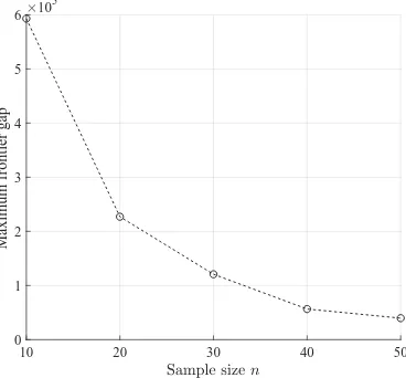
like O(n−1). This is shown in in Figure 8.2 which plots the maximum gap (over δ) between the
out-of-sample frontier and the true frontier under the true frontier for different values of n.
10 20 30 40 50
0 1 2 3 4 5 6
Maximum frontier gap
105
Figure 8.2. Gap between the out-of-sample frontier and true frontier asngets large.
Recall, in the previous section, we proposed the bootstrap frontier as an approximation to the
sample frontier. We next investigate how well the bootstrap frontier approximates the
the bootstrap frontier to equal the out-of-sample frontier exactly, it need only preserve therelative
shape of the out-of-sample frontier. As an example, suppose the bootstrap frontier matched the
out-of-sample frontier with the only difference being that it was double its size (in both the mean
and variance axis). In this scenario, the choice of δ should be the same when using either frontier
since the relative trade-off between mean and variance is identical. In light of this observation,
in Figures 8.3 (A), (B), and (C) we plot the normalized bootstrap and out-of-sample frontiers,
where the change in the mean and variance has been normalized to 1, for various sample sizes
n= 10,30,50, respectively. It is clear that as the sample size increases, the bootstrap frontier more
closely approximates the relative shape of the out-of-sample frontier.
8.2. Application 2: Portfolio Optimization. In our second application, we consider real monthly
return data from the “10 Industry Portfolios” data set of French [22]. The reward function is
ex-ponential utility of returns
f(x, R) =−exp−γR⊤x, (8.2)
wherex∈Rdis the portfolio vector (decision variables),R∈Rdis the vector of random returns, and
γ is the risk-aversion parameter. To simplify the experiments, we choose a risk-aversion parameter
γ = 1. For the purposes of this example, we impose a budget constraint 1⊤x= 1 and assume that
asset holdings are bounded, −1≤xi≤1, i= 1, ..., d.
We conduct the following experiment. We haved= 10 assets and are interested to see how robust
optimization and our approach for calibratingδ perform when we estimate the 10-dimensional joint
distribution with relatively few data points (n= 50, for the time period April 1968 to June 1972).
The robust portfolios will be tested on the empirical distributions for monthly returns of future 50
month windows, July 1972 to September 1976, October 1976 to December 1980 and January 1981
to March 1985 that do not overlap with the training set.
To begin, we solve the robust portfolio choice problem using the 50 monthly returns for the period
April 1968 to June 1972 for different values of δ and construct the robust mean-variance frontier
using the bootstrap procedure described in Algorithm 1. Figure 8.4 shows the associated bootstrap
robust mean-variance frontier, around which we also mark the +/−one standard deviations of the
bootstrap samples in both the mean and variance dimensions. Empirical optimization corresponds
to the point δ = 0, and as predicted by Theorem 6.1, there is significantly more reduction in the
0 0.1 0.2 0.3 0.4 0.5 0.6 0.7 0.8 0.9 1
Normalized variance of the reward
0 0.2 0.4 0.6 0.8 1 1.2
Normalized mean reward
(a) n= 10.
0 0.1 0.2 0.3 0.4 0.5 0.6 0.7 0.8 0.9 1
Normalized variance of the reward
0 0.2 0.4 0.6 0.8 1 1.2
Normalized mean reward
(b)n= 30.
0 0.1 0.2 0.3 0.4 0.5 0.6 0.7 0.8 0.9 1
Normalized variance of the reward
0 0.2 0.4 0.6 0.8 1 1.2
Normalized mean reward
(c) n= 50.
Figure 8.3. Bootstrap frontier vs out-of-sample frontier (with normalization). Both frontiers are scaled and normalized so that both the mean and variance equal 1 whenδ = 0 (i.e., empirical optimization) and 0 in the most robust case (δ= 100). We see that as n increases, the points on the frontier corresponding to the same values ofδ converge.
Calibration and Out-of-sample Tests: The bootstrap frontier estimates the the out-of-sample mean
and variance for different decisions and can be used to calibrate δ. For this example, the rate
of variance reduction relative to the loss in the mean is substantial for δ ≤ 5, but this begins to
diminish (and the cost of robustness increases) onceδexceeds 5. A value ofδbetween 2 and 5 seems
reasonable. While values ofδ >10 may be preferred by some, the balance clearly tips towards loss
in mean reward relative to variance reduction/robustness improvement. Note also that a classical
Variance of utility
Mean utility
Figure 8.4. Bootstrap robust mean-variance frontier for portfolio optimization generated using 50 months of monthly return data between April 1968 and June 1972.
select δ = 0 which corresponds to empirical optimization and completely nullifies all the benefits
of the robust optimization model.
It is also interesting to compare calibration using the bootstrap frontier with the decisions
ob-tained by solving robust optimization problems with “high confidence uncertainty sets”. The basic
idea behind this approach is to use uncertainty sets that include the true data generating model
with high probability, where the confidence level 1−α (typically 90%, 95%, or 99%) is a primitive
of the model. The use of uncertainty sets with these confidence levels is commonly advocated in
the robust optimization literature.
For a given statistical significance level 0< α <1, define an uncertainty set of the form
Uα={Q:H(Q|Pn)≤Qn(α)}, (8.3)
where H is some statistical distance measure and the threshold Qn(α) is the (1−α)-quantile of
the distribution ofH(Q|Pn) under the assumption that the data have the distribution Pn, i.e., the probability that the true data generating model lies in Uα is (1−α). Theα-parameterized “high
confidence uncertainty set” problem is then given by
max x Qmin∈Uα
EQ
f(x, Y)
. (8.4)
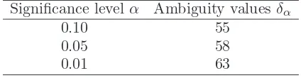
It can be shown that for anyαthere is a unique ambiguity parameter valueδα >0, for which the
solution of (8.4) coincides with our robust solutionx∗(δ
α). In Table 8.1 we report the corresponding
ambiguity parameter values δα for typical values of the significance levelα.
Table 8.1. Corresponding ambiguity parameter values δα for various traditional values of the significance levelα
Significance level α Ambiguity values δα
0.10 55
0.05 58
0.01 63
While robust decisions associated with the significance levels in Table 8.1 may or may not perform
well out-of-sample in this or any given application, it is clear that the range ofδα associated with
these significant levels is limited. This directly impacts the range of possible solutions available to
the decision maker, which in this example are concentrated on the “extremely conservative” region
of the bootstrap frontier (Figure 8.4). This approach cannot access a broad range of reasonable
solutions due to the nature of its parameterization.
We next analyze the out-of-sample performance of the robust solutions corresponding to δ =
1,2,3,5,10 obtained from our bootstrap frontier in Figure 8.4, the three “high confidence
uncer-tainty set” solutions of corresponding to δα = 55 (α = 0.10), δα = 58 (α = 0.05), δα = 63
(α = 0.01), and the empirical optimization solution corresponding to δ= 0. In particular, we test
each of the solutions on the empirical distributions for three out-of-sample test sets of data size
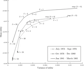
n= 50 that do not overlap with the training data; Figure 8.5 shows the out-of-sample performance.
Note that in the figure we report the mean and variance of the utility function f(x, R) defined in
(8.2), which is consistent with the framework of the robust optimization model in this paper.
Figure 8.5 consistently shows that as the value ofδ(“robustness”) increases from zero, the mean
performance degrades but the objective variability reduces, which is expected from our theory.
Consistent with the bootstrap frontier (Figure 8.4), the portfolios associated with “high confidence
uncertainty sets” have low variance though the impact on expected utility is substantial.
8.3. Application 3: Logistic Regression. As final application we apply robust optimization to
logistic regression which we evaluate on the WDBC breast cancer diagnosis data set [34].
The reward function for logistic regression is given by
0 0.002 0.004 0.006 0.008 0.01 0.012
Variance of utility
-0.99 -0.985 -0.98 -0.975 -0.97 -0.965 -0.96
Mean utility
Figure 8.5. Three out-of-sample mean-variance frontiers for the portfolio problem. The frontiers are the average mean and variance over test data sets of 50 months.
where Y ∈ {−1,1} is the binary label, Z is the vector of covariates, and x and x0 are decision
variables representing coefficients and intercept, respectively, of the linear model for classification.
Ordinary logistic regression is formulated as the maximization of the sample average of (8.5).
To demonstrate the out-of-sample behavior of robust maximum likelihood, we solve the
or-dinary/robust likelihood maximization problem using the first half of the WDBC breast cancer
diagnosis data set [34], i.e., 285 out of the 569 samples, and compute the log-likelihood and the
variance of the log-likelihood of the resulting model using the remaining half of the samples, i.e.,
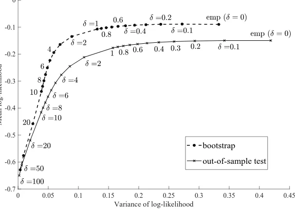
284 out of 569. Figure 8.6 shows both the the bootstrap frontier and the frontier obtained from
the out-of-sample test. Once again, that choices ofδ that deliver good out-of-sample log-likelihood
can be obtained using the bootstrap estimate of the robust frontier.
9. Conclusions
Proper calibration of DRO models requires a principled understanding of how the distribution
of the out-of-sample reward depends on the “robustness parameter”. In this paper, we studied
out-of-sample properties of robust empirical optimization and developed a theory for data-driven
0 0.05 0.1 0.15 0.2 0.25 0.3 0.35 0.4 0.45 Variance of log-likelihood
-0.7 -0.6 -0.5 -0.4 -0.3 -0.2 -0.1 0
Mean log-likelihood
bootstrap
out-of-sample test
Figure 8.6. Bootstrap frontier vs. out-of-sample test frontier with WDBC breast cancer diagnosis data set.
The out-of-sample test frontier shows the mean and variance of the log-likelihood of the second-half of the samples of the WDBC data set (i.e., 284 samples) on the basis of solutions obtained by using the first-half of those (i.e., 285 samples). Here, we used three attributes: no.2, no.24, and no.25 (out of 30 available covariates), which are found to be best possibly predictive in the paper [40]. To solve the optimization problems, we used RNUOPT (NTT DATA Mathematical Systems Inc.), a nonlinear optimization solver package.
“little bit of robustness” is a significant reduction in the variance of the out-of-sample reward while
the impact on the mean is almost an order of magnitude smaller. Our results imply that the
robustness parameter should be calibrated by making trade-offs between estimates of the
out-of-sample mean and variance and that substantial variance reduction is possible at little cost when
the robustness parameter is small. To calibrate the robustness parameter, we introduced the robust
mean-variance frontier and showed that it can be approximated using resampling methods like the
bootstrap. We applied the robust mean-variance frontiers to three applications: inventory control,
portfolio optimization and logistic regression. Our results showed that classical calibration methods
that match “standard” confidence levels (e.g. 95%) are typically associated with an excessively
large robustness parameter and overly pessimistic solutions that perform poorly out-of-sample,
while ignoring the variance and calibrating purely on the basis of the mean (a second-order effect)
can lead to a robustness parameter that is too small and a solution that misses out on the first-order
References
[1] Abu-Mostafa, Y.S., Magdon-Ismail, M., Lin, H.-L. 2012.Learning from Data. AMLbook.com.
[2] Ban, G.Y., El Karoui, N., Lim, A.E.B. 2016. Machine Learning and Portfolio Optimization.Management Science. Articles in Advance,https://doi.org/10.1287/mnsc.2016.2644.
[3] Ben-Tal, A., den Hertog, D., De Waegenaere, A., Melenberg, B., Rennen, G. 2013. Robust solutions of optimization problems affected by uncertain probabilities. Management Science. 59(2), 341–357.
[4] Ben-Tal, A., Nemirovski, A. 1998. Robust convex optimization.Mathematics of Operations Research. 23(4). 769– 805.
[5] Ben-Tal, A., El Ghaoui, L., Nemirovski, A. 2009.Robust Optimization. Princeton University Press. [6] Bergemann, D., Morris, S. 2005. Robust Mechanism Design.Econometrica, 73(6), 1771-1813.
[7] Bergemann D., Schlag, K. 2011. Robust monopoly pricing.Journal of Economic Theory, 146, 2527–2543. [8] Bertsimas, D., Gupta, V., Kallus, N. 2017. Data-driven robust optimization.Mathematical Programming. Online
First Articles,https://doi.org/10.1007/s10107-017-1125-8
[9] Bertsimas, D., Gupta, V., Kallus, N. 2014. Robust SAA. arXiv:1408.4445. (https://arxiv.org/abs/1408.4445). [10] Bertsimas, D., Litvinov, E., Sun, A.X., Zhao, J., Zheng, T. 2013. Adaptive robust optimization for the security
constrained unit commitment problem.IEEE Transactions on Power Systems, 28(1), 52–63. [11] Bertsimas, D., Sim, M. 2004. The price of robustness.Operations Research, 52(1), 35–53.
[12] Brown, D., De Giorgi, E., Sim, M. 2012. Aspirational preferences and their representation by risk measures. Management Science, 58(11), 2095–2113.
[13] El Ghaoui, L., Lebret, H. 1997. Robust solutions to least-square problems to uncertain data matrices. SIAM Journal on Matrix Analysis and Applications, 18, 1035–1064.
[14] Delage, E., Ye, Y. 2010. Distributionally robust optimization under moment uncertainty with application to data-driven problems.Operations Research, 58(3), 595–612.
[15] Doyle, J.C., Glover, K., Khargonekar, P.P., Francis, B.A. 1989. State-space solutions to standardH2 and H∞
control problems.IEEE Transactions on Automatic Control, 34(8), 831–847.
[16] Duchi, J.C., Namkoong, H. 2016. Variance-based regularization with convex objectives. arXiv:1610.02581v2. (https://arxiv.org/abs/1610.02581).
[17] Duchi, J.C., Glynn, P.W., Namkoong, H. 2016. Statistics of Robust Optimization: A Generalized Empirical Likelihood Approach. arXiv:1610.03425 (https://arxiv.org/abs/1610.03425).
[18] Efron, B., Tibshirani, R.J. 1994.An Introduction to the Bootstrap. Chapman & Hall.
[19] Ellsberg, D. 1961. Risk, Ambiguity and the Savage Axioms.Quarterly Journal of Economics, 75, 643-669. [20] Epstein, L.G. and T. Wang. 1994. Intertemporal Asset Pricing Under Knightian Uncertainty.Econometrica, 62,
283-322.
[21] Erdogan, E., G. Iyengar. 2006. Ambiguous Chance Constrained Problems and Robust Optimization, Mathemat-ical Programming, 107(1-2), 37–61.
[22] French, K.R. 2015. 10 Industry Portfolios. Posted December 2014, received April 2, 2015, http://mba.tuck.dartmouth.edu/pages/faculty/ken.french/Data_Library/det_10_ind_port.html.
[24] Gilboa, I. and D. Schmeidler. 1989. Maxmin Expected Utility with Non-unique Prior.Journal of Mathematical Economics, 18, 141–153.
[25] Gotoh, J., Kim, M.J., Lim, A.E.B. 2017. Robust empirical optimization is almost the same as mean-variance optimization. Submitted.
[26] Hansen, L. P., Sargent, T.J. 2001. Robust Control and Model Uncertainty. American Economic Review, 91, 60–66.
[27] Hansen, L.P., Sargent, T.J. 2008.Robustness. Princeton University Press, Princeton, New Jersey.
[28] Hastie, T., Tibshirani, R., Friedman, J. 2009.Elements of Statistical Learning (2ndEdition). Springer-Verlag.
[29] Jacobson, D.H. 1973. Optimal stochastic linear systems with exponential performance criteria and their relation to deterministic differential games.IEEE Transactions on Automatic Control, 18, 124–131.
[30] Kim, M.J., Lim, A.E.B. 2014. Robust multi-armed bandit problems.Management Science, 62(1), 264–285. [31] Klibanoff, P., Marinacci, M., Mukerji, S. 2005. A Smooth Model of Decision Making under Ambiguity.
Econo-metrica, 73(6), 1849–1892.
[32] Knight, F.H. 1921.Risk, Uncertainty and Profit, Houghton Mifflin, Boston, MA.
[33] Lam, H. 2016. Robust sensitivity analysis for stochastic systems. Mathematics of Operations Research, 41(4), 1248–1275.
[34] Lichman, M. (2013) UCI Machine Learning Repositoryhttp://archive.ics.uci.edu/ml. Irvine, CA: University of California, School of Information and Computer Science.
[35] Lim, A.E.B., Shanthikumar, J.G. 2007. Relative entropy, exponential utility, and robust dynamic pricing. Oper-ations Research, 55, 198–214.
[36] Lim, A.E.B., Shanthikumar, J.G., Shen, Z.J. 2006. Model uncertainty, robust optimization, and learning. TutO-Rials in Operations Research, 3, 66–94.
[37] Lim, A.E.B., Shanthikumar, J.G., Watewai, T. 2011. Robust asset allocation with benchmarked objectives. Mathematical Finance, 21(4), 643–679.
[38] Liu, J., Pan, J., Wang, T. 2005. An Equilibrium Model of Rare-Event Premia and its Implication for Option Smirks.Review of Financial Studies, 18, 131–164.
[39] Maenhout, P.J. 2004. Robust Portfolio Rules and Asset Pricing.The Review of Financial Studies, 17(4), 951–983. [40] O.L. Mangasarian, W.N. Street and W.H. Wolberg. 1995. Breast cancer diagnosis and prognosis via linear
programming. Operations Research, 43(4), 570–577.
[41] Peterson, I.R., James, M.R., Dupuis, P. 2000. Minimax optimal control of stochastic uncertain systems with relative entropy constraints.IEEE Transactions on Automatic Control, 45, 398–412.
[42] Shapiro, A., Dentcheva, D., Ruszczy´nski, A. 2014.Lectures on Stochastic Programming: Modeling and Theory, Second Edition. MOS-SIAM Series on Optimization.
[43] Uppal, R., Wang, T. 2003. Model misspecification and under-diversification.Journal of Finance, 58(6), 2465– 2486.
[44] Wu, D., Zhu, H., Zhou, E. 2017. A Bayesian Risk Approach to Data-driven Stochastic Optimization: Formula-tions and Asymptotics. arXiv:1609.08665. (https://arxiv.org/abs/1609.08665).
Appendix A. Appendix
A.1. Asymptotic normality: General results. We summarize results from [45] on the theory
of M-estimation that we use to characterize the asymptotic properties of robust optimization.
Let
x∗ := arg max x
n
EP
g(x, Y)o
,
xn := arg max x
n
EPn
g(x, Y) ≡ 1n
n X
i=1
g(x, Yi) o
.
The following result from [45] gives conditions under whichxn is asymptotically normal.
Theorem A.1. For every xin an open subset of Euclidean space, letx7→ ∇xg(x, Y)be a
measur-able vector-valued function such that, for everyx1 andx2 in a neighborhood ofx∗ and a measurable
functionF(Y) with EP[F(Y)2]<∞
k∇xg(x1, Y)− ∇xg(x2, Y)k ≤F(Y)kx1−x2k.
Assume that EPk∇2xg(x∗, Y)k2 <∞ and that the map x7→EP[∇xg(x, Y)]
is differentiable at a solution x∗ of the equation EP[∇
xg(x, Y)] = 0 with non-singular derivative
matrix
Σ(x∗) :=∇xEP[∇xg(x, Y)].
If EPn∇xg(xn, Y)
=oP(n−1/2), andxn→P x∗, then √
n(xn−x∗) = Σ(x∗)−1 1
√n
n X
i=1
∇xg(x∗, Yi) +oP(1).
In particular, the sequence√n(xn−x∗)is asymptotically normal with mean0and covariance matrix
Σ(x∗)−1E
P[∇xg(x∗, Y)∇xg(x∗, Y)′](Σ(x∗)−1)′.
Under conditions that allow for exchange of the order of differentiation with respect to x and
integration with respect to Y, we have
Σ(x) :=∇2xEP[g(x, Y)] =∇xEP[∇xg(x, Y)] =EP
∇2xg(x, Y)
Note however that Theorem A.1 does not require thatx7→g(x, Y) is twice differentiable everywhere
for Σ(x) to exist.
A.2. Proof of Proposition 5.1. Taylor series implies
f(x+δ∆, Yn+1) =f(x, Yn+1) +δ∆′∇xf(x, Yn+1) +
We obtain (5.2) by taking expectations and noting that ∆ and Yn+1 are independent. To derive
(5.3) observe firstly that
When ∆ is constant, the definition of a derivative implies (5.4) and the expansion of VP[f(x+
![Figure 1.1. Simulated mean reward—usual practice for calibration.the investor’s utility function values is taken over 50 bootstrap samples, attainingthe maximum atselection (ii) consists ofdata set at [34], and the average of the log-likelihood (y-axis) is](https://thumb-ap.123doks.com/thumbv2/123dok/2118373.1609601/3.612.95.520.76.241/simulated-practice-calibration-bootstrap-attainingthe-atselection-consists-likelihood.webp)