AUTOMATIC BUILDING EXTRACTION FROM LIDAR DATA COVERING COMPLEX
URBAN SCENES
Mohammad Awrangjeba,∗, Guojun Luaand Clive S. Fraserb
a
School of Information Technology, Federation University - Australia Churchill Vic 3842 Australia - (Mohammad.Awrangjeb, Guojun.Lu)@federation.edu.au b
CRC for Spatial Information, Dept. of Infrastructure Engineering, University of Melbourne Parkville Vic 3010, Australia - [email protected]
Commission IIIWG III/4
KEY WORDS:LIDAR, point cloud, segmentation, building, detection, roof, plane, extraction.
ABSTRACT:
This paper presents a new method for segmentation of LIDAR point cloud data for automatic building extraction. Using the ground height from a DEM (Digital Elevation Model), the non-ground points (mainly buildings and trees) are separated from the ground points. Points on walls are removed from the set of non-ground points by applying the following two approaches: If a plane fitted at a point and its neighbourhood is perpendicular to a fictitious horizontal plane, then this point is designated as a wall point. When LIDAR points are projected on a dense grid, points within a narrow area close to an imaginary vertical line on the wall should fall into the same grid cell. If three or more points fall into the same cell, then the intermediate points are removed as wall points. The remaining non-ground points are then divided into clusters based on height and local neighbourhood. One or more clusters are initialised based on the maximum height of the points and then each cluster is extended by applying height and neighbourhood constraints. Planar roof segments are extracted from each cluster of points following a region-growing technique. Planes are initialised using coplanar points as seed points and then grown using plane compatibility tests. If the estimated height of a point is similar to its LIDAR generated height, or if its normal distance to a plane is within a predefined limit, then the point is added to the plane. Once all the planar segments are extracted, the common points between the neghbouring planes are assigned to the appropriate planes based on the plane intersection line, locality and the angle between the normal at a common point and the corresponding plane. A rule-based procedure is applied to remove tree planes which are small in size and randomly oriented. The neighbouring planes are then merged to obtain individual building boundaries, which are regularised based on long line segments. Experimental results on ISPRS benchmark data sets show that the proposed method offers higher building detection and roof plane extraction rates than many existing methods, especially in complex urban scenes.
1. INTRODUCTION
Automatic extraction of buildings from remote sensing data is a prerequisite for many GIS (Geographic Information System) ap-plications, such as urban planning and 3D building modelling. Since airborne LIDAR systems provide an efficient way for rapid high resolution 3D mapping of the earth surface, much research currently focusses on automatic feature (buildings, trees, roads, ground etc.) extraction from LIDAR data. The ISPRS test project1 on urban object classification and 3D building reconstruction has given impetus to the process of evaluation and comparison of pro-posed methods on a common platform.
There are two test data sets in the ISPRS benchmark project: Vaigingen (VH) from Germany and Downtown Toronto (TR) from Canada. The VH data set represents a mixture of historic and res-idential buildings, with the historic buildings having a complex roof structure and the residential buildings a rather simple roof structure. Although there is a considerable amount of vegetation in this data set, the number of high-rise buildings is limited. In contrast, the TR data set is from the central business district of Toronto. This data set contains representative scene characteris-tics of a modern mega city in North America, including a mixture of low- and high-story buildings with a wide variety of rooftop structures. An example of such complex high-rise buildings is
∗Corresponding author.
1
Available at http://www2.isprs.org/commissions/comm3/ wg4/tests.html.
Figure 1: A complex urban scene, downtown Toronto.
shown in Figure 1.2 Consequently, the task of building detection and reconstruction in the TR data set is far more difficult than in the VH data set.
The complexity of the task of building extraction in the TR data set is not only due to complex roof structures, but also because buildings have varying heights that contribute significant shad-ows and occlusions. It is well known that shadshad-ows and occlusions are two major problems in feature extraction from aerial imagery.
2
Although shadows are not a problem in the LIDAR system, oc-clusions cause a large number of data gaps in the LIDAR point cloud. However, multiple passes from different angles by the LI-DAR system can overcome this problem by capturing data of the occluded areas. There is another problem that might be observed in LIDAR data, namely that in a modern mega city like Toronto, different types of materials are used both on the roof and walls of a building. Some of these materials are glass which may be trans-parent or semitranstrans-parent. As a consequence, there is a signifi-cant number of unexpected LIDAR points reflected from objects inside the building and under the rooftop. Many of these points may be considered as noise. This phenomenon adds difficulty in building extraction from LIDAR point clouds in cities.
This paper proposes a new building detection method using a novel segmentation technique for LIDAR point cloud data cov-ering complex urban scenes. The point cloud data is first divided into ground and non-ground points using a height threshold above the ground height. The non-ground points are mainly buildings and trees and these are further processed to remove the trees and to separate individual buildings. Points on walls can be removed by applying a plane fitting technique and by projecting data onto a dense grid. The remaining non-ground points are then divided into clusters based on height and local neighbourhood. The over-lapping points between the neghbouring planes are assigned to the appropriate planes based on their locality and the plane inter-section line. A rule-based procedure is then applied to remove tree planes, which are small in size and randomly oriented. The neighbouring planes are merged to obtain individual building re-gions. The building boundaries are regularised by adjusting small lines with respect to long lines.
2. RELATED WORK
Dorninger and Pfeifer (2008) proposed a comprehensive method for extraction, reconstruction and regularization of roof planes from LIDAR point clouds. Jochem et al. (2012) presented a roof plane segmentation technique from raster LIDAR data using a seed point based region growing technique. Oude Elberink and Vosselman (2009) used a target based graph matching approach that can handle both complete and incomplete laser data. Exten-sive and promising experimental results were shown on four data sets. Rau (2012) proposed a line-based roof model reconstruction algorithm, called TIN-Merging and Reshaping.
Awrangjeb and Fraser (2014a) proposed a region-growing method based on a plane-fitting technique using LIDAR point cloud data. Gerke and Xiao (2014) combined aerial imagery and LIDAR data to separately detect four object classes including buildings. Sohn et al. (2012) proposed a new algorithm to generalize noisy poly-lines comprising a rooftop model by maximizing a shape regular-ity (orthogonalregular-ity, symmetricregular-ity and directional simplications). Mongus et al. (2014) used a multi-scale decomposition of LI-DAR point cloud data to separate ground points and they applied a local surface fitting technique for extraction of planar segments. Awrangjeb et al. (2013) used roof edge and ridge lines from the aerial orthoimagery to define seed points for a region-growing technique applied on LIDAR point cloud data.
3. PROPOSED METHOD
Figure 2 shows the work flow of the proposed building extrac-tion technique. The proposed method first divides the input LI-DAR point cloud data into ground and non-ground points. The non-ground points, representing objects above the ground such
Figure 2: The proposed building extraction method.
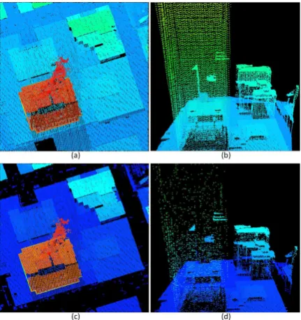
Figure 3: A sample scene from the Toronto data set: (a) LIDAR points, (b) 3D view, (c) non-ground points and (d) non-ground points after removal of wall points. In each figure, points at sim-ilar heights are shown using the same colour.
as buildings and trees, are further processed for building extrac-tion. Points on walls are removed from the non-ground points, which are then divided into clusters. Planar roof segments are ex-tracted from each cluster of points using a region-growing tech-nique. The extracted segments are refined based on the relation-ship between each pair of neighbouring planes. Planar segments constructed in trees are eliminated using information such as area, orientation and unused LIDAR points within the plane boundary. Points on the neighbouring planar segments are accumulated to form individual building regions. A new algorithm is proposed to regularise the building boundary. The final output from the pro-posed method will be individual buildings and roof planes (points and 3D boundaries).
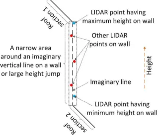
Figure 4: LIDAR points reflected from a narrow area around an imaginary line on a wall or large height jump.
are described using this sample scene.
3.1 Finding non-ground points and removing wall points
The non-ground points can be easily separated from the ground points using a bare-earth DEM (Digital Elevation Model). If a bare-earth DEM is not available, one can be generated from the LIDAR point cloud data. We assume that the bare-earth DEM is given as an input to the proposed method. For each LIDAR point, the corresponding DEM height is used as the ground heightHg. A height thresholdTh=Hg+hc, wherehcis a height constant that separates low objects from higher objects, is then applied to the LIDAR data. In this study,hc= 1m has been set (Awrangjeb and Fraser, 2014a). Figure 3(c) shows the non-ground points for the sample scene.
A 2D neighbourhood, for example, Delaunay triangles or Voronoi neighbourhood, is usually considered in any region growing seg-mentation technique. A large number of unexpected triangles or neighbourhood points can be found for the points on a roof with the points on its walls. Since this paper aims for an ef-fective segmentation of individual roof planes, the wall points are first removed by applying a plane fitting technique and by projecting data on a dense grid as follows. A fictitious horizon-tal planeℑis formed. Considering the length and width of the test area to bela(Easting) andwa(Northing), the following four points can be used to constructℑ:(1,1,1),(la,1,1),(1, wa,1)
and (la, wa,1), where a constant height of 1 m is considered. For each non-ground LIDAR pointP, its neighbouring point set Sn={Qi}is obtained, where each neighbourQiresides within a distanceHdfromPand has a maximum height difference ofVd withP. The value of the horizontal distance thresholdHdis set at twice the maximum point-to-point distance (dm) in the input LIDAR data (Awrangjeb et al., 2013). Considering the maximum slope (with respect toℑ) for a roof plane is 75◦, the value of the vertical distance thresholdVdis set atdm×tan(75◦). Sn in-cludesPand if|Sn| ≥3, a planeζpis constructed forP. If the angle betweenζpandℑis at most32π, thenζpis determined as a
vertical plane andPis removed as a wall point.
The above procedure removes a large number of points reflected from walls. However, some of the points on walls may still sur-vive, especially those which reside far away from each other or get reflected from different planes of a wall. The surviving wall points, which reside within the area close to an imaginary verti-cal line on a wall can be removed easily. Figure 4 shows such wall points which are far away (more thanHd) from each other. In order to remove these points, all the surviving points are pro-jected onto a dense grid of resolution 0.25 m (Awrangjeb et al., 2012). Assuming that the grid resolution is less than the LIDAR
Figure 5: (a) Clusters of points for the sample scene in Figure 3 and (b) extracted planar segments.
point density (i.e.,dm>0.25m), this projection will transfer all points within a narrow area close to an imaginary vertical line to the same grid cell. If a grid cell has more than one projected point, points that are at the top and bottom of the line are kept and others are removed. For illustration, the red coloured points in Figure 4 are removed, but the light blue coloured points are preserved. Figure 3(d) shows the non-ground LIDAR points after the removal of wall points. As can be seen in the figure, points that are far away from each other or are reflected from different planes of a wall can not be removed. However, it will be unlikely that a vertical plane is extracted from these surviving wall points.
3.2 Point clustering
All the non-ground points obtained after removal of wall points are now processed to generate clusters of points based on height. Initially, all these points are not assigned to any clusters. Consid-ering the maximum LIDAR height as the current height, points at this height (within a specified tolerance) are found and one or more clusters are initialised depending on their locality. Then each of the cluster is extended until no points can be added to the cluster. Points in each cluster are marked so that they are not as-signed to another cluster. Once all the clusters initialised from the current height are finalised, the points that are not yet assigned to any clusters are then processed to generate more clusters. The next current height will be the maximum height of these unas-signed points.
Let the current maximum height be hm and the set of points that has similar height (i.e., withinhm±Tf, whereTf = 0.1m (Awrangjeb et al., 2013) to allow the error in LIDAR generated heights) is Sc. One or more clustersξi, wherei≥1, are ini-tialised usingScbased on the locality. For a pointP ∈ξi, there is at least one neighbouring pointQin the same cluster such that the 2D Euclidean distance|P.Q| ≤Hd. IfP andQare in two different clusters then|P.Q|> Hd.
In order to extend a clusterξi, letRbe a neighbour ofP, where P ∈ξi butRhas been neither assigned to any cluster nor yet designated as a wall point. Ris considered to be a neighbour of P, if|P.R| ≤Hdand their height difference is withinVd. Ris added toξi, which is iteratively extended until noRis found as a neighbour ofP.
ξiis considered a valid cluster if it is larger than 1 m2 in area. To obtain the area of a cluster, its points are projected onto an initially white maskMwof resolution 0.25m (Awrangjeb et al., 2012). For each point projected at location(x, y)ofMw, all the pixels within an×nneigbourhood are made black. The value ofnis determined based ondmand the resolution ofMwsuch that all the pixels corresponding to an individual building, roof section or plane become black. The area ofξi is thus roughly estimated by counting the number of black pixels multiplied by the pixel size.
Figure 5(a) shows a 3D view of all the clusters for the sample scene in Figure 3. Compared to the wall points in Figure 3(d), Figure 5(a) shows that the points on walls are not assigned to any clusters for the sample scene in Figure 3(a). Trees with small canopy can also be removed in this clustering technique.
3.3 Roof plane extraction
Planar roof segments are extracted from each cluster of points. By using the Delaunay triangulation algorithm, a natural bourhood of points in the cluster can be generated. The neigh-bourhood of a point P consists of the points Qi, 1≤i≤n, where each lineP Qiis a side of a Delaunay triangle. In order to avoid points which are far away fromP, the following condition is applied: |P Qi| ≤Td. The coplanarity ofP is decided using its neghbouring points following the procedure in Awrangjeb and Fraser (2014a). Points within a roof plane are found to be copla-nar and those along the boundary of a plane are generally found to be non-coplanar.
For each cluster, let the two sets of the non-ground LIDAR points beS1, containing all the coplanar points, andS2, containing the
rest (non-coplanar). The first planar segment can now be ini-tialised using a coplanar pointP ∈S1and its neighbours. This
new planar segment is extended using the neighbouring points fromS1andS2. Once the extension is complete, all the coplanar
points in the extended planar segment are marked so that none are latter used for initiating another planar segment. As a result, the points inS2, which mainly reside along the plane boundaries,
can be used by more than one extracted plane. The second planar segment is grown by using an unused coplanar point (fromS1).
The iterative procedure continues until no coplanar point remains unused.
Figure 5(b) shows all the extracted planes for the sample scene. Since two extracted planes may have some points in common, es-pecially along the plane intersection or when a plane is extracted twice or more times. In order to refine the extracted planes, the following rules are applied: First, if two planes share the major-ity of the plane points they are considered to be coincident planes (i.e., a plane is multiply extracted) and they are merged. Second, if two planes are parallel, each of the common pointsP is as-signed to the plane with which it has a smaller normal distance. Third, for two non-parallel planes, ifP is coplanar then two an-gles are estimated between its normal and the two plane normals. P and its neighbours are then assigned to the plane with which the angle is smaller. Fourth,Pcan also be assigned based on its locality, i.e., assigned to the nearest plane. Finally, the remaining common points are assigned based on their locations with respect to the plane intersection line.
In order to remove false-positive planes, mostly constructed on trees, a rule-based procedure is applied. For an extracted LI-DAR plane, its area, straight line segments along its boundary, and neighbourhood information, as well as any LIDAR spikes within its boundary, are used to decide whether it is a false alarm. For a given point on the extracted LIDAR plane, the mean height
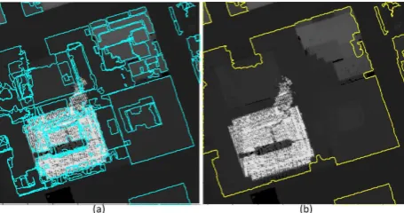
Figure 6: (a) Extracted plane boundaries for the sample scene in Figure 3 and (b) extracted building boundaries. Both are shown overlaid on a digital surface model for the sample scene.
Figure 7: Extracting a 3D plane boundary: (a) LIDAR points on the plane, (b) Canny edge around a mask of resolution 0.25 m and (c) boundary after assigning only height values from the nearest LIDAR points to boundary in (b).
difference with its neighbouring points is also used. This height difference is large for a tree plane, but small for a roof plane. The average height difference for a plane is estimated from individual height differences within the plane. A LIDAR plane fitted on a tree is usually small in size and there may be some LIDAR spikes within its boundary. Moreover, there may be a large number of unused (i.e., not on any of the extracted planes) LIDAR points within the boundary of a tree plane. The number of points used by the extracted planes is usually low on a tree cluster, but high on a building cluster. Moreover, there may be some long straight line segments (at least 3m long. minimum building width (Awrang-jeb et al., 2010)) along the boundary of a roof plane. Figure 6(a) shows the final extracted roof planes.
3.4 Building boundary extraction and regularisation
In order to obtain the boundary of an extracted plane, LIDAR points on the plane are used. Figure 7(a) shows the points for an extracted plane. A binary mask of resolution 0.25 m is gen-erated, as shown in Figure 7(b). Then, the Canny edge around the black shape in the mask is extracted. Since the edge is a 2D boundary, the height values from the nearest LIDAR points are assigned to the edge points. Fig. 7(c) shows the extracted plane boundary. Figure 6(a) shows the boundaries of the extracted roof planes from the sample scene.
All the LIDAR points from the neighbouring roof planes are now merged in order to obtain an individual building segment. The building boundary is thus extracted following the same procedure discussed above. Figure 6(b) shows the building boundaries for the sample scene.
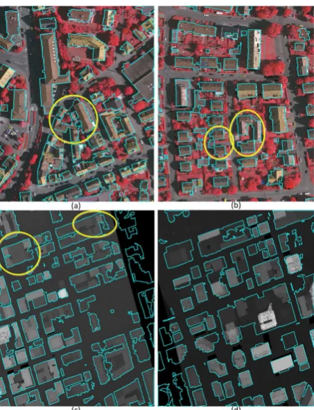
Figure 8: Building footprints overlaid on orthoimagery or on dig-ital surface models: (a) Area 1, (b) Area 3, (c) Area 4 and (d) Area 5. Yellow coloured ellipses show examples of merged buildings.
line is then fit using the LIDAR points within the boundary seg-ment between two consecutive corners. Lines which are at least 6 m in length, twice the minimum building length are kept fixed. Other lines are rotated to make them either parallel or perpendicu-lar to the nearest fixed lines. Perpendicuperpendicu-lar lines are then added in between successive parallel lines. Finally, the intersection points of consecutive lines are obtained and the nearest LIDAR point heights are assigned to the intersection points to obtain the regu-larised building boundary. Figure 8 shows the reguregu-larised build-ing footprints for four test areas.
4. PERFORMANCE STUDY
In the performance study conducted to assess the proposed ap-proach, all five test areas adopted by the ISPRS benchmark project were employed. The objective evaluation followed the system in Rutzinger et al. (2009) adopted by the ISPRS benchmark project. In this system, three categories of evaluations (object-based, pixel-based and geometric) have been considered. A num-ber of metrics have been used in the evaluation of each category. While the object-based metrics, completeness, correctness, qual-ity and under- and over-segmentation errors, estimate the perfor-mance by counting the number of objects (buildings or planes in this study), the pixel-based metrics, completeness, correct-ness and quality, show the accuracy of the extracted objects by counting the number of pixels. In addition, the geometric metric (root mean square error, RMSE) indicates the accuracy of the ex-tracted boundaries and planes with respect to the reference enti-ties. The definitions of these indices can be found in the literature (Rutzinger et al., 2009, Awrangjeb et al., 2010, Awrangjeb and Fraser, 2014b). In the ISPRS benchmark, the minimum areas for large buildings and planes have been set at 50 m2and 10 m2, re-spectively. Thus, the object-based completeness, correctness and
quality values will be separately shown for large buildings and planes.
4.1 Data sets
The first data set is from Vaihingen (VH) in Germany (Cramer, 2010). There are three test areas in this data set and each area is covered with a point density of 4 points/m2. Area 1 is situated in the centre of the town of Vaihingen. It is characterized by dense development consisting of historic buildings having rather com-plex shapes, and it also has some trees. Area 2 is characterized by a few high-rise residential buildings that are surrounded by trees. Area 3 is purely residential, with detached houses and many sur-rounding trees. The number of buildings (larger than 2.5 m2) in these three areas is 37, 14 and 56, and the corresponding number of planes is 288, 69 and 235, respectively.
The second data set covers the central area of the City of Toronto (TR) in Canada. This ‘Downtown Toronto’ data set contains rep-resentative scene characteristics of a modern mega city in North America, including a mixture of low- and high-story buildings with a wide variety of rooftop structures, and street and road fea-tures. There are two areas selected from this data set and each has a point density of 6 points/m2. The first area (Area 4) contains a mixture of low and high, multi-story buildings, showing various degrees of shape complexity in rooftop structure and rooftop fur-niture. The scene also contains different urban objects including cars, trees, street furniture, roads and parking lots. The second area (Area 5) represents a typical example of a cluster of high-rise buildings. The scene contains shadows cast by high buildings, under which various types of urban objects (e.g., cars, street fur-niture, and roads) can be found. The number of buildings (larger than 2.5 m2
) in these two areas is 58 and 38, and the correspond-ing number of planes is 968 and 641, respectively.
4.2 Experimental results and discussion
The evaluation results are presented for building detection and roof plane extraction separately.3
4.2.1 Building detection Table 1 shows the object-based eval-uation results and Table 2 shows the pixel-based and geomet-ric evaluation results. Figures 9 and 10 depict the pixel-based performance in all five areas. They also show some complex cases, where the proposed method either failed to detect some small buildings (or parts of large buildings) or mistakenly de-tected some other objects.
The proposed method performed well in all five test areas. When all the buildings are considered, the average completeness and correctness in object-based evaluation were about 89%, with an average quality of 80% (Table 1). As shown in Table 2, the pro-posed method performed better in pixel-based evaluation, where completeness, correctness and quality values were 2 to 3 % higher than those in the object-based evaluation.
However, the proposed method failed to detect some small build-ings. Two such examples are shown by yellow circles in Fig-ure 9(f). As shown in FigFig-ure 9(e), the method also failed to ex-tract certain complex roof structures. Some building parts that are close to the ground are also missed. The building part within the black rectangle in Figure 9(f) is less than 1 m above the ground. Another such example is shown in Figure 10(c). Figures 10(d)-(e) show two opposite scenarios, where although the structures
3
Table 1: Object-based evaluation of building detection results. Object-based: Cm = completeness, Cr = correctness and Ql = quality (Cmb,Crb and Qlb are for buildings over 50 m2
) in percentage. Segmentation errors: M = over-segmentation,N = under-segmentation andB= both over- and under-segmentation.
Area Cm Cr Ql Cmb Crb Qlb M/N/B
1 89.2 91.4 82.3 100 100 100 0/6/0
2 85.7 92.3 80 100 100 100 0/2/0
3 83.9 97.9 82.5 97.4 100 97.4 0/8/0
4 100 83.6 83.6 100 94.9 94.9 1/11/0
5 86.8 78.6 70.2 91.4 94.1 86.5 0/1/0
Avg 89.1 88.8 79.7 97.8 97.8 95.8 0.2/5.6/0
Table 2: Pixel-based and geometric evaluation of building detec-tion results. Pixel-based: Cmp= completeness,Crp = correct-ness andQlp = quality in percentage. Geometric: planimetric accuracy with respect toRpe= extracted and Rpr = reference buildings in metre.
Area Cmp Crp Qlp Rpe Rpr
1 88.1 90 80.3 0.95 1
2 87.1 94 82.6 0.9 0.81
3 87.7 89 79.1 0.75 0.96
4 95.1 91.1 87 0.96 1.07
5 96.7 93.2 90.3 0.89 0.93
Avg 90.9 91.5 83.9 0.89 0.95
Table 3: Object-based evaluation of plane extraction results. Object-based: Cm= completeness,Cr = correctness andQl= quality (Cmb,CrbandQlbare for planes over 10 m2) in percent-age. Segmentation errors: M = over-segmentation,N = under-segmentation andB= both over- and under-segmentation.
Area Cm Cr Ql Cmb Crb Qlb M/N/B
1 66 91.7 62.3 85.7 97.5 83.9 17/22/11
2 71 90.7 66.2 85.4 100 85.4 11/2/0
3 73.2 89.2 67.3 91.9 99.1 91.2 7/34/2
4 70.2 78.3 58.8 87.1 89 78.6 180/30/84
5 67.9 80.7 58.4 88.2 84.3 75.8 96/26/57
Avg 69.7 86.1 62.6 87.7 94 83 62.2/22.8/30.8
are higher than the surrounding ground, they are found as false positive.
When buildings larger than 50 m2 are considered, the method showed the maximum performance in Areas 1 and 2. However, in Area 3 a large building was missed due to missing LIDAR data, as illustrated in Figure 9(d). In both Areas 4 and 5, some low objects were detected as shown in Figure 10(b). In Area 5, some low buildings were also missing. Consequently, in Areas 3 to 5, the proposed method did not perform the maximum for large buildings.
In Areas 1, 3 and 4 there are many under-segmentation errors as indicated in Table 1. These errors were due to merging of nearby buildings, as shown within yellow coloured ellipses in Figure 8. In terms of planimetric accuracy (Table 2), the proposed method showed better accuracy with respect to the extracted footprints than with respect to the reference data. The overall error was within 1 to 2 times the maximum point spacing in the input LI-DAR point cloud data.
4.2.2 Roof plane extraction Table 3 shows the object-based evaluation results and Table 4 shows the pixel-based and geomet-ric evaluation results. Figures 11 and 12 illustrate the extracted plane boundaries for four test areas.
Figure 9: Building detection in the Vaihingen data set: (a) Area 1, (b) Area 2 and (c) Area 3. Some complex cases are shown in (d) to (f). Yellow = true positive, blue = false negative and red = false positive pixels.
Figure 10: Building detection in the Toronto data set: (a) Area 4 and (b) Area 5. Some complex cases from (a) and (b) are shown in (c) to (e). Yellow = true positive, blue = false negative (FN) and red = false positive (FP) pixels.
In object-based evaluation (Table 3), the proposed method per-formed better in the Vaihingen than in the Toronto data sets. Among three Vaihingen areas, it performed the best in Area 3, which is a residential area, followed by Areas 2 and 1. Between the two Toronto areas, the method performed slightly better in Area 4 than in Area 5. A similar performance trend was observed for planes larger than 10 m2in area.
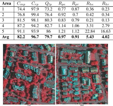
Table 4: Pixel-based and geometric evaluation of plane extraction results. Pixel-based:Cmp= completeness,Crp= correctness and Qlp = quality in percentage. Geometric: planimetric accuracy with respect toRpe= extracted andRpr= reference planes and height error with respect toRhe= extracted andRhr= reference planes in metre.
Area Cmp Crp Qlp Rpe Rpr Rhe Rhr
1 74.4 97.9 73.2 0.77 0.87 0.36 0.23
2 76.8 99.4 76.4 0.92 0.7 0.42 0.34
3 81.5 98.1 80.3 0.83 0.79 0.21 0.13
4 87.2 94.2 82.7 1.14 1.06 3.31 2.79
5 91.1 93.9 86 1.21 1.12 22.84 16.63
Avg 82.2 96.7 79.7 0.97 0.91 5.43 4.02
Figure 11: Extracted roof planes in the Vaihingen data set: (a) Area 1 and (b) Area 3.
the benchmark data sets and the method missed many of these. The large number of over-segmentation errors indicates that the method did not work well for complex roof structures, especially in Areas 4 and 5. Moreover, a high number of under-segmentation errors in all areas, except in Area 2, is clear evidence that the method merged a large number of neighbouring small planes with big planes.
In pixel-based evaluation (Table 4), in terms of completeness and quality, the method performed best in Area 5 followed by Areas 4, 3, 2 and 1. Among all test areas, it showed the best correctness in Area 2, followed by Area 3. In Areas 4 and 5 many false planes were extracted, as shown by red coloured pixels in Figure 10(a)-(b).
The planimetric accuracy was similar to that in building detection results, approximately 1 to 2 times the maximum point spacing in the input LIDAR point cloud. In terms of height accuracy, the method showed better performance in the Vaihingen data set than in the Toronto data set. In Area 5, it showed a significant height error.
On average, the proposed method showed better performance in pixel-based evaluation than in object-based evaluation. While in object-based evaluation the completeness, correctness and qual-ity values were 70%, 76% and 63%, respectively, in pixel-based evaluation they were 82%, 97% and 80%, respectively. Thus, it is evident that although the proposed method is capable of recognis-ing all LIDAR points on complex buildrecognis-ing roofs, it suffers from a large number of segmentation errors.
4.3 Comparative performance
In this section, the results from the proposed method are com-pared with those from existing methods that exploit LIDAR data as an input source. The methods being compared in this study are chosen such that they have been tested at least against the TR data
Figure 12: Extracted roof planes in the Toronto data set: (a) Area 4 and (b) Area 5.
set, which represents a modern city.4 As usual, the comparisons are shown separately for building detection and roof extraction.
4.3.1 Comparing building detection performance In build-ing detection, in Areas 1 to 3 the proposed method always showed better completeness, in both object- and pixel-based evaluation, than Mongus et al. (2014). In Area 3, the proposed method showed significantly better object-based completeness than Mongus et al. (84% vs 70%). But Mongus et al. showed 4 to 9% better correctness in some cases, specially in Areas 1 and 3. In Area 4, Mongus et al. showed better correctness values (3 to 11%) than the proposed method. However, in Area 5 the proposed method offered 3 to 17% better object-based and pixel-based correctness. Nevertheless, Mongus et al. is a semiautomatic method as it has to tune parameter values for different test data sets. For exam-ple, the area threshold was set at 25 m2
for the VH data set and 100 m2for the TR data set, which is also an indication that their approach is unable to detect small buildings such as garages and garden sheds.
In terms of object- and pixel-based correctness and complete-ness and also when buildings larger than 50 m2
are considered, the proposed method (in most cases, except an object-based cor-rectness value in Area 4) offered better performance than Gerke and Xiao (2014) in Areas 4 and 5. In the TR data set, while the object-based correctness values were around 80% by the pro-posed method, those by Gerke and Xiao were significantly lower (e.g., less than 30% in Area 5). A similar performance difference was found in Area 2: while Gerke and Xiao offered significantly lower object-based correctness values (12 and 42% using Markov model and random tree, respectively), the proposed method of-fered a high correctness of 92%. In Area 3, while the proposed method offered an object-based correctness of 98%, Gerke and Xiao showed only 63% correctness when the Markov model was used for unsupervised classification.
4.3.2 Comparing roof extraction performance In Area 4, in most cases the proposed method offered 2 to 10% better cor-rectness and completeness than Rau (2012), which showed 2% more pixel-based correctness than the proposed method (80 vs 78%). The proposed method also showed better planimetric and height accuracy in this area. In Area 5, in terms of completeness and correctness, while the proposed method offered 1 to 3% bet-ter object-based performance, Rau offered 2 to 3% betbet-ter pixel-based performance. In this area, although the proposed method offered better planimetric accuracy (1.1 m vs 1.8 m) than Rau, it showed higher height errors. In Areas 1 to 3, while the proposed method offered better height accuracy, Rau in general offered bet-ter pixel-based completeness and correctness. It should be noted
4
that Rau is a semiautomatic method and the structure lines need to be manually extracted from the stereo-pair, whereas the proposed method is fully automatic.
In Area 5, in both object- and pixel-based evaluations, while the proposed method offered 2 to 3% better completeness than Sohn et al. (2012), the latter showed 2 to 4% better correctness. In Area 4, in most cases Sohn et al. gave better performance than the proposed method, while the proposed method showed better object-based completeness and planimetric accuracy. In Areas 1 to 3, in most cases Sohn et al. again offered better performance than the proposed method. The proposed method showed better completeness in Area 2 and better height accuracy in all 3 areas.
In all test areas, while the proposed method suffered from more over-segmentation errors, Rau (2012) and Sohn et al. (2012) had more under-segmentation errors.
5. CONCLUSION
A method for segmentation of LIDAR point cloud data for au-tomatic detection and extraction of building rooftops has been proposed. Experimental results have shown that the proposed method is capable of yielding higher building detection and roof plane extraction rates than many existing methods, especially in complex urban scenes, as exemplified here by downtown Toronto.
However, since the method uses LIDAR data alone, the planimet-ric accuracy is limited by the LIDAR point density. At present, the method does not incorporate smoothing of the boundaries of extracted planar segments. Moreover, it will not work on curved roofs. Since the involved evaluation system (Rutzinger et al., 2009) is a threshold-based evaluation system, a bias-free eval-uation using an automatic and threshold-free system (Awrangjeb and Fraser, 2014b) would be useful for more reliable experimen-tal results. Future work will look at the development of a regular-isation procedure to smooth roof plane boundaries and to recon-struct building roof models. The integration of image data will also facilitate better object extraction where LIDAR information is missing. An extension of the proposed method could be the use of higher density point cloud data (e.g., a low density LIDAR point cloud complemented by a DSM derived from dense image matching) and thus the curved surfaces could be better approxi-mated.
ACKNOWLEDGEMENTS
Dr. Awrangjeb is the recipient of the Discovery Early Career Researcher Award by the Australian Research Council (project number DE120101778). The Vaihingen data set was provided by the German Society for Photogrammetry, Remote Sensing and Geoinformation (DGPF) (Cramer, 2010). The authors would like to acknowledge the provision of the Downtown Toronto data set by Optech Inc., First Base Solutions Inc., GeoICT Lab at York University, and ISPRS WG III/4.
REFERENCES
Awrangjeb, M. and Lu, G., 2008. Robust image corner de-tection based on the chord-to-point distance accumulation tech-nique. IEEE Transactions on Multimedia 10(6), pp. 1059–1072.
Awrangjeb, M., Ravanbakhsh, M. and Fraser, C. S., 2010. Au-tomatic detection of residential buildings usingLIDARdata and multispectral imagery. ISPRS Journal of Photogrammetry and Remote Sensing 65(5), pp. 457–467.
Awrangjeb, M., Zhang, C. and Fraser, C. S., 2012. Building de-tection in complex scenes thorough effective separation of build-ings from trees. Photogrammetric Engineering & Remote Sens-ing 78(7), pp. 729–745.
Awrangjeb, M., Zhang, C. and Fraser, C. S., 2013. Automatic extraction of building roofs usingLIDARdata and multispectral imagery. ISPRS Journal of Photogrammetry and Remote Sensing 83(9), pp. 1–18.
Awrangjeb, M. and Fraser, C. S., 2014a. Automatic Segmentation of RawLIDARData for Extraction of Building Roofs. Remote Sensing 6(5), pp. 3716–3751.
Awrangjeb, M. and Fraser, C. S., 2014b. An automatic and threshold-free performance evaluation system for building ex-traction techniques from airborneLIDARdata. IEEE Journal of Selected Topics in Applied Earth Observations and Remote Sens-ing, doi: 10.1109/JSTARS.2014.2318694.
Cramer, M., 2010. TheDGPFtest on digital aerial camera evalua-tion - overview and test design. Photogrammetrie Fernerkundung Geoinformation 2, pp. 73–82.
Dorninger, P. and Pfeifer, N., 2008. A comprehensive automated 3D approach for building extraction, reconstruction, and regu-larization from airborne laser scanning point clouds. Sensors 8, pp. 7323–7343.
Gerke, M. and Xiao, J., 2014. Fusion of airborne laserscanning point clouds and images for supervised and unsupervised scene classification. ISPRS Journal of Photogrammetry and Remote Sensing 87, pp. 78–92.
ISPRSbenchmark, 2013. Benchmark data sets and test re-sults. http://www2.isprs.org/commissions/comm3/wg4/ results.html(last date accessed: 15 Jan 2014).
Jochem, A., H¨ofle, B., Wichmann, V., Rutzinger, M. and Zipf, A., 2012. Area-wide roof plane segmentation in airborneLIDAR
point clouds. Computers, Environment and Urban Systems 36(1), pp. 54–64.
Mongus, D., Luka˘c, N. and ˘Zalik, B., 2014. Ground and building extraction fromLIDARdata based on differential morphological profiles and locally fitted surfaces. ISPRS Journal of Photogram-metry and Remote Sensing 93(7), pp. 145–156.
Oude Elberink, S. and Vosselman, G., 2009. Building reconstruc-tion by target based graph matching on incomplete laser data: analysis and limitations. Geodetski Vestnik 9(8), pp. 6101–6118.
Rau, J. Y., 2012. A line-based3Droof model reconstruction al-gorithm: TIN-merging and reshaping (TMR). In: ISPRS Annals of the Photogrammetry, Remote Sensing and Spatial Information Sciences, Vol. I-3, Melbourne, Australia, pp. 287–292.
Rutzinger, M., Rottensteiner, F. and Pfeifer, N., 2009. A compari-son of evaluation techniques for building extraction from airborne laser scanning. IEEE Journal of Selected Topics in Applied Earth Observations and Remote Sensing 2(1), pp. 11–20.
Sohn, G., Jwa, Y., Jung, J. and Kim, H. B., 2012. An implicit regularization for3Dbuilding rooftop modelling using airbourne